1. Introduction

The demand for architectural and structural design for high-rise residential buildings has increased as a result of rapid global urbanization [1,2]. The structural design process includes conceptual, detailed, and construction drawing design, with conceptual design relying heavily on immense knowledge and experience and having a significant impact on subsequent design decisions [3]. Furthermore, due to its manual and iterative engineering features, the traditional structural design process can be inefficient, failing to meet the current demands for fast and high-quality conceptual design of shear wall systems [4]. As a result, intelligent and automated structural design methods that can learn from previous design data and conduct high-performance conceptual design are critical. There has been an emerging effort to develop deep learning-based structural design methods to generate structural design based on architectural drawings [4-6]. These promising methods are becoming versatile design approaches for the future.

In automated building design, optimization methods, such as evolutionary algorithms, topology optimization, and swarm intelligence, are widely used and significantly improve the design performance and qualities [7-14]. However, these methods are based on expert system methodologies and optimization algorithms, and they still have limitations. Because it is difficult to effectively and explicitly define the structural design-related variables and design rules in the expert system methodologies, they are not suitable for complex structural design. For designs based on optimization algorithms, it is difficult to properly formulate the corresponding objective function and boundary function according to the design rules. Furthermore, the low efficiency of optimization algorithms cannot satisfy today's architectural-structural design efficiency requirements in the schematic design phase. More importantly, neither method makes full use of existing structural design data, such as the existing efficient and good-quality designs. This could result in repeated and unnecessary work, so it should be reconsidered and addressed, especially with the cutting-edge technologies of artificial intelligence. In comparison, intelligent generative structural design, such as deep neural network-based structural parametric determination method [5,6] and GAN-based layout design method [4], can learn from the experience in existing design documents directly and efficiently. In this case, not only the features of well-performing designs can be inherited and re-applied, but also the engineers will be provided with a good reference design instantly, which significantly speeds up the entire scheme design process.

Deep learning is the engine of intelligent generative structural design. It is traditionally a data-driven learning method heavily dependent on the data quantity and quality [15-19]. Since the introduction of StructGAN, a generative adversarial network (GAN)-based automated structural design method [4], feedback from case studies and subject-matter experts has prompted further improvement taking into account the physical behavior of the structure. Recently, physics-enhanced methods became popular because they improved the training quality of neural networks and the reliability of their output, helping neural networks learn from empirical and physical rules [20-24]. Moreover, a data-physics-driven intelligent design method for RC frame structures was also developed [25]. Hence, based on related studies, this study attempts to improve StructGAN by leveraging the physics-enhanced methods.

This study proposes StructGAN-PHY, a physics-enhanced GAN, and applies it to the structural design. The proposal enables an intelligent generative design that learns from a design database while being informed by assessing the physical performance by a surrogate model based on structural dynamics. After the physics-enhanced training, StructGAN-PHY can quickly generate a structural design that meets the architectural and physical requirements. This study introduces a physics-enhanced generative structural design framework in Section 2, with the physics calculator and estimator as primary innovations. Section 3 presents the implementation and performance of the physics calculator. Section 4 presents the network model and effectiveness of the physics estimator. Finally, case studies to evaluate the performance of StructGAN-PHY are presented in Section 5.

2. Physics-enhanced generative structural design method

Physics-enhanced GAN is an innovative architecture of the deep neural network by developing the physics estimator and embedding it into the conventional GAN. Hence, the generator is guided by the discriminator and physics estimator simultaneously (Figure 1(a)). Based on Physics-enhanced GAN, The proposed physics-enhanced generative structural design method consists of two primary steps, as shown in Figure 1.

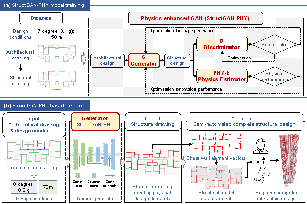
Figure 1   Physics-enhanced generative structural design method

a. Step 1 is the training of the StructGAN-PHY model (Figure 1(a)). The existing structural design drawings and their corresponding design conditions are collected to establish the training and test datasets for the StructGAN-PHY model.

b. Step 2 is the StructGAN-PHY-based design (Figure 1(b)). The well-trained StructGAN-PHY model, whose training process is shown in Figure 1(a), generates a semantic structural design image using the architectural drawing and design conditions as input, as shown in Figure 2(a). The intelligent design structural image is then converted to a structural design model (e.g., the ETABS analysis model), using the proposed semi-automated complete structural scheme design method. Note that the semantic design image is a pre-processed drawing in which the critical design components, such as the shear wall, infill wall, window, and gate elements, are extracted from the original design drawings and coded by different colors [4].

The preliminary design process can be significantly improved with the help of StructGAN-PHY. An architect without a structural design background can easily obtain the corresponding structural scheme using an architectural floorplan image. Structural engineers, on the other hand, can use the proposed method to generate efficient structural design schemes for optimized designs, speeding up the design process by 90 times. Additionally, this data-driven method allows for the learning and efficient application of previous design outcomes, avoiding duplicate or similar work.

The StructGAN-PHY model is created by incorporating the physics estimator into the GAN model [4,26,27]. The physics estimator is a neural network-based surrogate model, trained by the generated structural drawing and labeled with the corresponding physical performance indicator, which estimates the physical performance according to the generated structural drawing. The physical performance indicators are outputted by the physics calculator, which is created based on the physics-driven structural analysis model. Moreover, the generator of StructGAN-PHY is optimized by the physics-enhanced loss, after which it manages to master the physical mechanism. The detailed StructGAN-PHY model and corresponding training method are presented in the following sections.

StructGAN-PHY can improve the design reliability of physical performance and reduce the dependence on high-quality data. Moreover, it can generate thoughtful structural designs even without training data under the relevant design conditions. Thus, physics-enhanced generative structural designs possess competitive advantages, including high efficiency, universality, and practicality.

2.1 Datasets

This study collected approximately 150 architectural and structural drawings and their corresponding design conditions from more than 10 prestigious architectural and structural design institutes in China. Among them, 17 sets of data include detailed structural design models.

In this study, data preprocessing is essential for neural networks to extract features and learn critical elements in design drawings. Using the data preprocessing method of Liao et al. [4], this study applies the semanticization method to extract the primary design features from the original design drawings, including the shear wall, infill wall, window, and gate elements (Figures 2(a)). In addition, the calculation of the structural dynamic response requires critical design conditions (i.e., seismic design intensity and structural height). The datasets are generated based on the above primary feature extraction method. Typical datasets are shown in Figures 2(b) and 2(c). The training data are labeled with the structural drawings generated by engineers (quantity: 135, augmented to 540 by flipping and mirroring) [4], while 24 sets of test data have no corresponding labels.

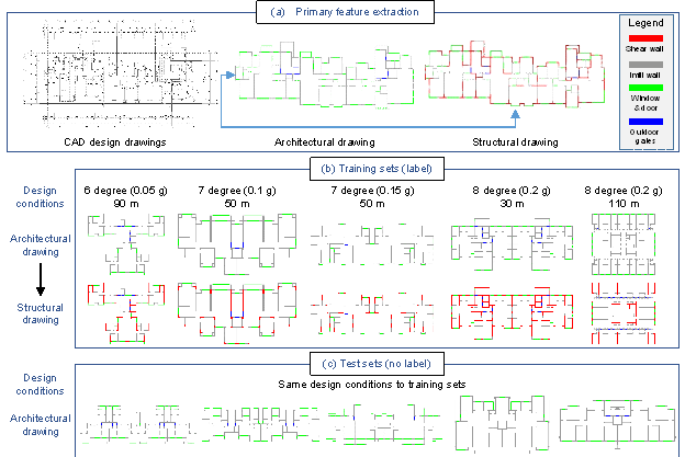
Figure 2   Datasets. (a) Primary feature extraction of design drawings, (b) typical training sets, and (c) typical test sets. In the design conditions, for example, 6-degree (0.05 g) denotes that the seismic design intensity is 6-degree and that the corresponding peak ground acceleration (PGA) of the design basis earthquake (i.e., 10% probability of exceedance in 50 years) is 0.05 g. In design drawings, the red (RGB = (255, 0, 0)), gray (RGB = (132, 132, 132)), green (RGB = (0, 255, 0)), and blue (RGB = (0, 0, 255)) colors denote the structural shear wall, nonstructural infill wall, indoor window, and outdoor gate, respectively

2.2 Physics-enhanced GAN

As shown in Figure 3, the physics-enhanced GAN (StructGAN-PHY) consists of five components, including the (1) generator, (2) discriminator, (3) physics calculator, (4) physics estimator, and (5) physics-enhanced loss of the generator and data loss of the discriminator. The main contributions of this study are the physics calculator, estimator, and physics-enhanced loss.

(1), (2) Generator and discriminator. These two neural networks are established based on Wang et al. [27] and Liao et al. [4]. The generator is composed of convolutional networks for image feature extraction and deconvolutional networks for new image generation. The discriminator extracts image features and distinguishes between real and fake.

Figure 3   Physics-enhanced GAN

(3) Physics calculator (details are presented in Section 3). The output tensor from the generator networks is detached and converted into an array for image generation. The structural elements can be identified based on the image, and a corresponding structural analysis model is developed. The critical dynamic response and physical performance (e.g., seismic inter-story drift ratio) are obtained by analyzing the model. Furthermore, the crucial physical performance used in the structural design is related to the structural design requirements and codes. For example, owing to the high risk of earthquakes in China, an intensive seismic design is required for every building [28,29]. Therefore, the seismic inter-story drift ratio [30,31] is the most critical and dominant physical factor, which is used as the physical mechanism in this study. Seismic design intensity and structural height are adopted as the design conditions because they are regarded as the most critical for the seismic effect [4,28,29,32]. Moreover, the proposed method also applies to other design requirements (e.g., wind-load-governed structural design [9]).

(4) Physics estimator (details are presented in Section 4). The physics calculator is incompatible with the neural networks, which makes the output results of the physics calculator less helpful in optimizing the parameters of the generative network. Hence, this study develops a neural network-based surrogate model in the same computational graph as the generator, ensuring that the physical performance can efficiently guide the training of the generator. Moreover, the generator-output structural drawings and calculator-output physical performance are stored as datasets for training the physics estimator. A well-trained estimator is then used to optimize the generator parameters. The widely used ResNet18 model [33,34] is used as the estimator and outputs the physics loss (L_G-PHY).

(5) Physics-enhanced loss. L_G-PHY, L_G-img, and L_D-GAN are the physics loss, image generation loss, and discrimination loss, respectively. The generator loss (L_G) is a weighted combination of L_G-PHY and L_G-img.

Loss functions are critical for optimizing network parameters. The physics-enhanced generator loss and discriminator loss are calculated using Equations (1) and (2), respectively.

,                                                                                                                                    (1)

,                                                                                                                                                                        (2)

where L_G-img is the image generation loss, shown in Equation (3), L_G-PHY is the physics loss, output by the physics estimator, ω_img and ω_PHY are the weights of L_G-img and L_G-PHY, respectively, as shown in Equation (4), and L_D-GAN is the discriminator loss [27].

,                                                                                                                   (3)

where L_G-GAN, L_G-FM, and L_G-VGG are different types of image generation losses, and λ_FM is the corresponding weight [4,27]. L_G-img is mainly used in the early training process for image generation, which helps optimize the quality of the generator synthesis images.

The proposed method calculates the generator loss (L_G) as a weighted sum of L_G-img and L_G-PHY by considering the physics loss. According to Equation (4), the corresponding weights are set to change linearly in the training process, which ensures gradient stability of the parameter optimization and prevents the gradient from exploding or vanishing. ω_img decreases from 1 to 0.1, while 1 is the recommended initial value of ω_img during the training for image generation [4]; a value of 0.1 is set to ensure sufficient image quality. On the other hand, L_G-PHY is mainly in the range of [0, 1] (details are shown in Subsection 3.3); its weight ω_PHY increases from 0 to ω_PHYmax. The appropriate ω_PHYmaxis discussed in Subsection 4.2, which indicates that [1, 3] is the optimal range.

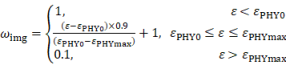
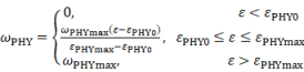
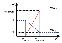
where ε is the current training epoch, ε_PHY0 is the epoch of using the physics estimator to output L_G-PHY, ε_PHYmax is the epoch of the image generation weight stopping to decrease, and ω_PHYmax is the maximum weight of L_G-PHY.

2.3 Training method of physics-enhanced GAN

Based on the above physics-enhanced GAN and its loss function, a network training method is proposed. The training process is shown in Figure 4, while the corresponding pseudocode is shown in Appendix A, which consists of three primary stages.

(1) Stage 1: Training for image generation. When ε < ε_PHY0 (the current training epoch is smaller than the epoch of training the physics estimator), the generator synthesizes structural drawings according to the input architectural drawing, while the discriminator distinguishes the synthetic structural drawing. The physics calculator outputs the physical performance of this synthetic structural drawing. The structural drawing and performance are stored in the training sets for the estimator.

(2) Stage 2: Training of the physics estimator. When ε = ε_PHY0, based on the training sets in Stage 1, the physics estimator is trained to precisely estimate the physical performance.

(3) Stage 3: Physics-enhanced training of the generator. When ε > ε_PHY0, the generator outputs structural drawings and the discriminator judges them. During this process, the well-trained physics estimator in Stage 2 estimates the physics loss (L_G-PHY) of the drawings. The parameters of the generator are then optimized with the weighted sum of the physics loss and image loss (Equation (1)).

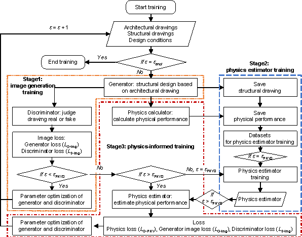
Figure 4   Training process of the physics-enhanced GAN

2.4 Physical performance evaluation method

The similarity between synthetic and ground-truth images is a widely used indicator for synthetic image quality evaluation [4,35,36]. However, a synthetic design that is less similar to the ground truth design does not necessarily indicate inferior performance. Hence, this study uses physical performance, rather than similarity, as the most critical indicator for structural design.

Physical-performance-based evaluation methods are proposed in this study, including (1) an multi-degree-of-freedom (MDOF)-model-based simplified evaluation method. The shear wall elements are extracted from the structural drawing using the method described in Subsection 3.1. The key parameters of the MDOF model are then determined. Subsequently, the MDOF model is established and analyzed. The simplified model is efficient, reasonable, and applicable for a wide range of designs [18,37-41]. (2) Finite-element (FE)-based refined evaluation method. Based on the extracted shear wall elements, engineers design the floor structure, apply loads, and analyze using FE software (e.g., ETABS [42]). Based on the complete design, precise results are available for a detailed evaluation of a typical structure.

3. Physical performance calculator

A physics calculator is developed in this study to evaluate the physical performance of a structural drawing and use it to guide the GAN training. The components of the physics calculator are illustrated in Figure 5, including Step 1 (convert image tensor to an array), Step 2 (obtain coordinates of structural components from images), Step 3 (build the structural analysis model), and Step 4 (conduct the physical performance analysis). In Step 1 and Step 2, conversion of pixel drawing to vector data is realized with the OpenCV package [43] (see Appendix B). In Step 3, the critical computational model is the MDOF model, which is widely used, accurate, and highly efficient [18,37-41] (see Subsections 3.1–3.3). In Step 4, the structural analysis is conducted in terms of the structural dynamics with the NumPy package [44].

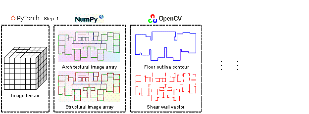
Figure 5   Physical performance calculation

3.1 MDOF model establishment

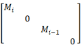
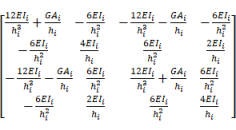
The shear wall structural system is primarily designed to resist lateral loads (e.g., seismic loads). Hence, this study uses the MDOF flexural-shear model, which is widely used in seismic analysis [18,37-41]. The conceptual MDOF model is shown in Figure 5. The corresponding computational story mass and stiffness matrices are shown in Equations (5) and (6), respectively. The story flexural stiffness (EI_i) and shear stiffness (GA_i) determine the structural dynamic response, which requires further study on parameter calibration (Subsection 3.2). Since shear wall residence is the main focus of this study and its structural layout is comparatively regular, the computation of lateral deformations can be decoupled along the x and y directions, neglecting torsional deformations [37].

,                                                                                                                                                         (5)

,                                                                                                                  (6)

where M_i, EI_i, GA_i, and h_i are the mass, flexural stiffness, shear stiffness, and height of the ith story, respectively.

In a simplified analysis, all shear wall elements can be approximately considered with a consistent horizontal deformation, based on the in-plane action of the rigid floor diaphragm assumption [9,32]. Moreover, the stiffness amplification effect of the beam and floor should also be considered. Hence, the story flexural stiffness (EI_i) can be calculated using Equation (7), where EI_i is the summation of the flexural stiffness of all shear walls on the ith story, multiplied by the amplification coefficient (λ_EI) of the floor structural system.

,                                                                                                                                                                    (7)

where λ_EI is the story flexural stiffness amplification coefficient, which is strongly related to the wall density and structural height. EI_i^j is the flexural stiffness of the jth shear wall component along its neutral axis.

Furthermore, because of the complexity of the structural shear deformation behavior, the story shear stiffness cannot be directly obtained by summarizing the shear stiffness of all shear wall units. Hence, this study uses the nondimensional parameter α_eq as the flexural-shear coefficient, which is used to estimate GA_i with EI_i [37],

,                                                                                                                                                            (8)

where α_eq is the flexural shear coefficient related to the wall density and H_struct is the structural height.

3.2 Parameter calibration of the MDOF model

In the MDOF model, three critical parameters cannot be directly obtained from the shear wall vectors in Figure 5: (1) the wall thickness (t_wall) for the inertia moment, (2) amplification coefficient of story flexural stiffness (λ_EI), and (3) flexural-shear coefficient (α_eq) for the story shear stiffness. From existing studies, only empirical values of the range of α_eq are provided [37], with few methods available to determine the values for these coefficients. Hence, this study proposes calibration of these parameters based on the structural design data and analysis model, as shown below.

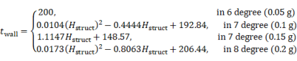
(1) Wall thickness (t_wall). In this study, wall thickness data are collected from approximately 150 structural design drawings with different design conditions, and then used to train a regression model for the wall thickness. Based on the Chinese seismic design code [29], the wall thickness is, in general, positively correlated to the building weight (represented by the structural height of the building) and seismic loads (indicated by the seismic design intensity). Hence, the datasets are grouped based on seismic design intensities, and then fitted using linear or quadratic curves. The resulting regression models for the wall thickness as a function of the structural height are shown in Figure 6(a) and Equation (9). Moreover, in practical applications, the wall thickness must also satisfy the axial compression ratio requirements under the self-weight and seismic load [29]. Hence, the wall thickness is determined by the envelope of regression and constrained by the mechanical computation results, which must also meet the modulus requirement (i.e., the thickness is a multiple of 20 mm).

,                                                     (9)

where t_wall denotes the wall thickness (unit: mm), H_struct is the structural height, and 6-degree (0.05 g), etc., are seismic design intensities (PGA corresponding to a 10% exceedance probability in 50 years) (see Figure 2).

(2) Calibrations of the story flexural stiffness amplification coefficient (λ_EI) and flexural shear coefficient (α_eq). In this study, 17 groups of design data are collected, including refined FE models using ETABS [42] and PKPM [45]. λ_EI and α_eq of the corresponding MDOF models are calibrated iteratively until the physical performance of the MDOF models, including the dynamic characteristics and inter-story drift ratio, converge to those of the refined FE models.

The amplification of the story flexural stiffness is mainly caused by the contribution of the floor system (including the coupling beam, frame beam, and floor). A parametric analysis indicates that λ_EI is highly sensitive to the wall density (ρ_wall) and structural height (H_struct). A higher ρ_wall and lower H_struct correspond to a smaller influence from the floor system. Hence, (ρ_wall / H_struct) is defined as the independent variable to fit the amplification factor (λ_EI). Moreover, the flexural shear coefficient (α_eq) primarily affects the shear deformation of the structure. The parametric analysis reveals that the wall density (ρ_wall) is most sensitive to α_eq. At a higher ρ_wall, the shear-dominant deformation transforms to the flexural-dominant deformation mode. Therefore, ρ_wall is used to fit the flexural shear coefficient (α_eq). The regression results for λ_EI and α_eq are shown in Figure 6(b) and Equations (10)–(12).

,                                                                                                                                 (10)

,                                                                                                                                              (11)

,                                                                                                                                                  (12)

where ρ_wall is the wall density in one direction, H_struct is the structural height,  is the length summation of all shear walls in one direction, and  is the equivalent structural plan length in one direction.

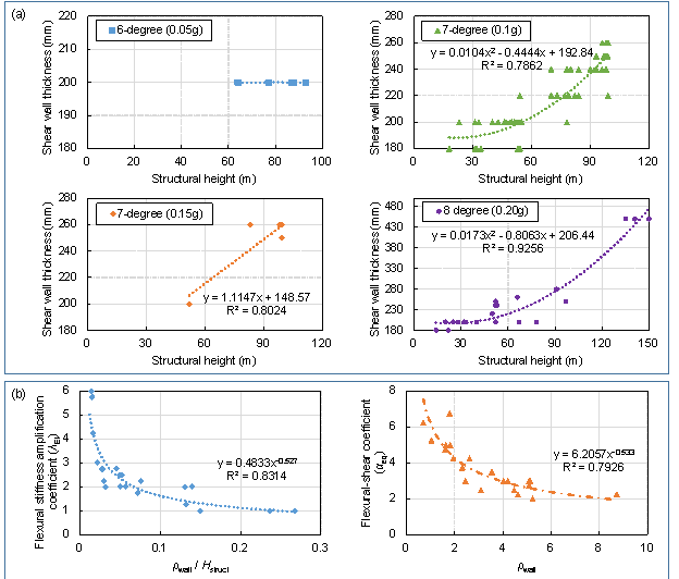
Figure 6   Calibration of the critical parameters for the structural stiffness matrices. (a) Shear wall thickness (where 6-degree (0.05 g), etc., denote the seismic design intensity (see Figure 2)), (b) flexural stiffness amplification coefficient (λ_EI), and flexural-shear coefficient (α_eq)

Table 1      Comparison of physical performances and computational efficiencies of MDOF and refined models

(3) MDOF model accuracy. Based on the calibration of λ_EI and α_eq in Step (2), this study quantifies the accuracy of the MDOF model. Using the collected refined FE models (e.g., the ETABS models) as benchmarks, the physical performance differences between the MDOF and refined models are calculated. The results are shown in Table 1, which indicates a difference in the performance of approximately 10%. The design experience survey of competent engineers shows that the difference in the inter-story drift ratio of 10% at the structural scheme stage does not have a significant impact on the detailed structural design. Additionally, the computational time of the ETABS model is approximately 600 times that of the MDOF model, which indicates that the use of the FE method for the structural analysis in the neural network training process can be intractable. Consequently, the MDOF model can efficiently optimize the neural network parameters using physical information within an acceptable error.

3.3 Physical performance indicator

In this study, a structural analysis is efficiently conducted based on the MDOF model. For structural design dominated by seismic loads, modal response spectrum analyses can be used to obtain the structural seismic deformation and inter-story drift ratio [29]. Through the structural response analysis, the maximum inter-story drift ratio (d_maxdrift) is mainly within [0.1‰, 2‰]. Furthermore, the structural deformation performance indicator (p_drift) is calculated using Equation (13). The equation indicates that, within the main interval of d_maxdrift, if d_maxdrift exceeds the drift limit, the indicator increases faster with d_maxdrift such that the current design is less preferred. Note that this statement is valid because most values of p_drift are in the range of [0, 1]. Finally, this study defines the physical performance (p_PHY) to be represented by p_drift, where a smaller value denotes a better physical performance.

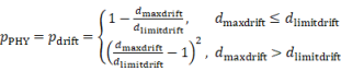
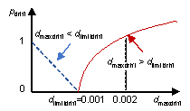
where d_limitdrift = 0.001 is the drift limit specified by the design code [29].

4. Physical performance estimator

Conventional physics-enhanced neural networks are realized by developing a physics-enhanced loss function. The corresponding physics-enhanced loss is calculated in the computational graph of neural networks so that the gradient can be automatically calculated and backpropagated for network parameter optimization [20-25]. However, for the structural performance calculation discussed in Section 3, neither the computational process matches the neural network computational graph nor the function for the structural performance is differentiable, preventing the physics mechanism from training the neural networks. Hence, in this study, an estimator is developed, which is a neural network-based surrogate model, to efficiently include physics loss into the generator loss and train the generator.

4.1 Neural networks of physics estimator

For the physics-enhanced GAN in this study, the physics estimator is the most substantial component that requires a rigorous comparison and selection from various networks. Widely used deep neural networks include the VGG and ResNet models [46]. Therefore, VGG16, VGG19 [47], ResNet18, ResNet34, and ResNet50 models [33,34] are used as physics estimators. The detailed training process for the estimator is shown in Stage 2 of Figure 4. The training sets for the estimator are established, where the generator outputs structural design drawings as the samples, and the calculator outputs their physical performances as labels. In total, there are 26800 sets of training data and 17800 sets of test data (training:test = 6:4). L1 loss is used as the loss function in the estimator training, as shown in Equation (14). The training and test of the estimator indicate that the estimator can accurately estimate the physical performance.

,                                                                                                                     (14)

where  is the estimator output physical performance indicator and  is the calculator output physical performance indicator.

Subsequently, the trained estimator is used in the physical mechanism learning process of the generator. The physics loss of the generator in the training process and generator test results are illustrated in Figure 7. As shown in Figure 7(a), different estimator networks have different effects on the physical mechanism learning. VGG network models have small effects on the training of the generator, while ResNet network models significantly help decrease the generator's physics loss. Figure 7(b) shows the physical performance (p_PHY) of the generated structural drawings, where a lower p_PHY corresponds to a better performance of the generator. The test results also reveal that the ResNet models effectively optimize the generator in physics-enhanced training. Consequently, the best ResNet18 model is used as the estimator.

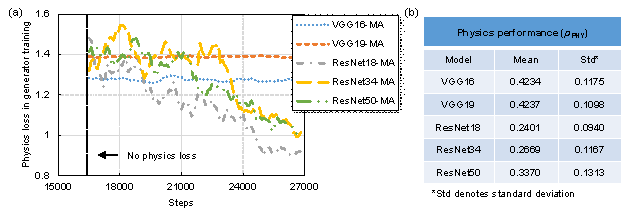
Figure 7   Guidance for generator training by different physics estimators. (a) Physics loss of the generator during the physics-enhanced training and (b) physical performance (p_PHY) of test designs by the physics-enhanced generator, shown in Equation (13)

4.2 Key parameter analysis

The networks and training method of the physics-enhanced GAN (introduced in Section 2) show that the parameters ε_PHY0 and ω_PHYmax are critical for the physical performance of the physics-enhanced GAN. Hence, a parametric analysis is conducted.

(1) ε_PHY0 in Equation (4) is the epoch of training the physics estimator, which determines the number of training data for the physics estimator. A large value of ε_PHY0 indicates that the estimator training process has sufficient training data, but an excessively large ε_PHY0 could also induce a negative effect on the estimator accuracy, as it may introduce similar or duplicate structural drawings in the training sets.

(2) ω_PHYmax in Equation (4) is the maximum weight of the physics loss, which determines the influence of the physical performance on the generator training process. A higher ω_PHYmax leads to more significance on the physics mechanism, but an unnecessarily large ω_PHYmax can induce an excessive physical influence and degrade the quality of the generated structural drawing.

The parametric analysis results are illustrated in Figure 8. As shown in Figure 8, when ε_PHY0 and ω_PHYmax are chosen within certain ranges, the generator exhibits a high performance of the structural design with robustness. Therefore, the recommended range for ε_PHY0 is [20, 30], while the recommended range for ω_PHYmax is [1, 3]. Note that when the datasets or estimator networks are different, the optimal ε_PHY0 and ω_PHYmax are recommended to be obtained via a parametric analysis.

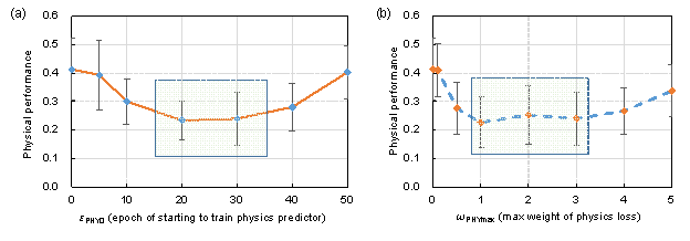
Figure 8   Critical parametric analysis results (the physical performance (p_PHY) is obtained by Equation (13), where a lower indicator value corresponds to a better performance). (a) Physical performance (mean and standard deviation) affected by ε_PHY0 and (b) physical performance (mean and standard deviation) affected by ω_PHYmax

5. Case studies

5.1 Case studies under different design conditions

Using the good-performing physics-enhanced generative structural design method, several case studies are conducted, where the first studies investigate various design conditions. The physical performance of 135 data points in the training set is analyzed via the MDOF-model-based simple evaluation method (Subsection 2.4). The training datasets are grouped based on the seismic design intensity and structural height [4]. Detailed information on the training data and corresponding physical performance are shown in Table 2.

To evaluate the performance of the proposed algorithm (i.e., StructGAN-PHY), it is compared with the generative structural design models without the physics-enhanced scheme (i.e., StructGAN). The corresponding training process considering different design conditions is shown in Figure 9. In StructGAN, the corresponding data are used for training if available; otherwise, the data for the adjacent design condition are used for training. In StructGAN-PHY, all training data are utilized. After the training process, both StructGAN and StructGAN-PHY models are tested using 24 architectural design drawings and evaluated with the MDOF model, as shown in Table 2.

As shown in Table 2, the structural physical performance of StructGAN-PHY is considerably better than that of StructGAN. When the training data are adequate (in terms of quantity and quality), the well-trained StructGAN can be efficient, such as Group 14 (8-degree (0.2 g), 40 - 60 m). However, when the data are scarce, such as Group 18 (8-degree (0.3 g), 40 - 60 m), the training data quality dominates the performance of StructGAN, causing significant under-fitting and performance degradation. In contrast, in the training process of StructGAN-PHY, the physical performance calculation can supply additional physical constraints to help the parametric optimization of the generator, which helps reduce the negative effect caused by the shortage and limitation of data quality and quantity.

Consequently, StructGAN-PHY effectively breaks through data limitations in the data-driven structural design method. With physics enhancement, the designs of StructGAN-PHY can better meet the design conditions, even when the data are insufficient. Overall, several case studies under different design conditions reveal that the physical performance of the StructGAN-PHY designs is 44% better than that of StructGAN designs.

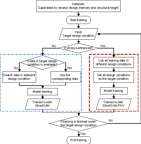
Figure 9   Training method of StructGAN and StructGAN-PHY under various design conditions

Table 2     Physical performance of the training datasets and test results (the physical performance (p_PHY) is obtained by Equation (13), where lower indicator values correspond to better performances)

*std: standard deviation

5.2 Case studies of typical refined design

The above case studies are conducted mainly via an evaluation method using the MDOF model. To further validate the performance of StructGAN-PHY, two refined structural model analyses are conducted and StructGAN-PHY is compared with StructGAN as well as competent engineers. The analysis method uses the FE-model-based evaluation method described in Subsection 2.4. These two cases are not used in the training and test processes. The case names and design conditions are defined as follows: (1) Case 8-degree-98m, where the seismic design intensity is set to 8-degree (0.2 g), while the structural height is set to 98 m, and (2) Case 7-degree-75m, where the seismic design intensity is set to 7-degree (0.1 g), while the structural height is set to 75 m. For StructGAN-PHY and StructGAN, the complete structural scheme designs are conducted using the method described in Subsection 2.4. Engineers conducted the design via an iterative and time-consuming design optimization process.

(1) The design results of the engineers, StructGAN-PHY, and StructGAN are shown in Figure 10. The structural design of StructGAN-PHY is quite similar to the design of engineers, with highly consistent shear wall layout positions and dimensions (i.e., length), which is significantly better than that of StructGAN. In contrast, Case 8-degree-98m by StructGAN has fewer shear wall elements than those of engineers and StructGAN-PHY, while Case 7-degree-75m by StructGAN has more shear wall elements.

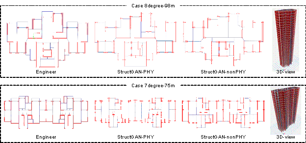
Figure 10 Comparison of structural designs of engineers, StructGAN-PHY, and StructGAN

(2) Furthermore, structural dynamic analyses are conducted, as shown in Table 3 and Figure 11. Regarding the comparison of the dynamic characteristics, in terms of critical translation periods, the design by StructGAN-PHY is similar to the engineer-optimized design (with an average difference of approximately 6%), while the designs by StructGAN exhibit a higher discrepancy (with an average difference of approximately 21%). As for the maximum inter-story drift ratio, the design generated by StructGAN-PHY is similar to the engineer-optimized design (with an average difference of approximately 9%) and conforms to the limit of the Chinese design code (i.e., 1/1000). On the other hand, the maximum inter-story drift ratio of the StructGAN design is quite different from that of the engineers' design (with an average difference of approximately 37%) as well as from the code limit.

In Case 8-degree-98m, less shear wall is generated in the design by StructGAN, inducing a small lateral stiffness and large deformation (50% larger than the design code limit), which is regarded as unsafe. On the other hand, in Case 7-degree-75m, the design by StructGAN has considerably more shear wall, resulting in over-conservativeness due to the inter-story drift ratio 50% below the code limit. Therefore, the data-driven method StructGAN strongly relies on data quality and quantity, which induces an unsatisfactory generalization ability, while the physics-enhanced method StructGAN-PHY can effectively overcome the deficiency caused by lack of knowledge from inadequate data.

Table 3      Comparison of structural design performances and design efficiencies of engineers, StructGAN-PHY, and StructGAN

* The design efficiency of engineers is mainly obtained through investigation by engineers, while the StructGAN-PHY design process is completed on a standard computer (central processing unit: Intel(R) Core(TM) i5-4590; random-access memory: 8 GB; Operating system: Windows 10).

(3) Finally, Table 3 compares the design efficiencies of StructGAN-PHY and engineers. StructGAN-PHY is 90 times faster than the engineer's design method. Moreover, the physical performances of the designs generated by StructGAN-PHY and engineers are relatively similar, with differences of approximately 6% in structural characteristics and 9% in the maximum inter-story drift ratio.

In summary, StructGAN-PHY can conduct structural design with high efficiency, quality, and intelligence.

Figure 11 Comparison of seismic inter-story drift ratios of engineers, StructGAN-PHY, and StructGAN. The mean difference in maximum inter-story drift ratio between StructGAN-PHY and engineers is 9%, while that between StructGAN and engineers is 37%

6. Conclusions

This study proposes a physics-enhanced generative structural design method (StructGAN-PHY) by developing surrogate physics models to train GANs. StructGAN-PHY overcomes the deficiency of the data-driven structural design method and generates structural designs that satisfy the physical demands. The conclusions of this study can be summarized as follows.

(1) The physics-enhanced GAN and corresponding training method are proposed, in which physics loss is fused into the data loss function. Through the physics-enhanced training process, StructGAN-PHY effectively learns the physical mechanism of structural design.

(2) A physics calculator was developed, which converts the pixel design drawing to an MDOF model and calibrates the critical parameters of the MDOF model. Within seconds, an MDOF structural model can be generated and analyzed. This highly efficient physical analysis method is applicable to the training of deep neural networks.

(3) A neural network-based surrogate model for physical performance estimation was developed, which effectively enabled the physical performance calculation to be compatible with neural network training. A physics calculator was used to train the physics estimator. The estimator provides physics loss for generator training, which successfully conducts automatic gradient calculation and backpropagation of the physics loss.

(4) Case studies indicated that the design performance of StructGAN-PHY was 44% better than that of StructGAN, which is 90 times faster in the complete design stage than the competent engineers, with a difference in physical performance of approximately 10%.

Although physics-enhanced GAN shows potential advantages, it is mainly recommended for the preliminary design stage and requires further processing, such as detailed structural design, before being used as a structural drawing. The error in the intelligent design process still needs to be identified.

Furthermore, in future studies, the precision of converting pixel images to structural component vectors, as well as the accuracy of physics-driven and data-driven surrogate models, should be improved; then, it is also necessary to consider the influence on shear wall layout design induced by architectural design, structural beams and slabs, vertical loads, and other factors; and finally, it is challenging to consider all of these factors at the same time. As a result, a combination of StructGAN-PHY and evolutionary algorithms could be used to optimize the generated preliminary design while taking into account the complex physical constraints.

Acknowledgment

Reference

[1]    CTBUH. Tall buildings in 2019: Another record year for supertall completions. CTBUH Research 2019. https://www.skyscrapercenter.com/research/CTBUH_ResearchReport_2019YearInReview.pdf

[2]    Perez RI, Carballal A, Rabuñal JR, García-Vidaurrázaga MD, Mures OA. Using AI to simulate urban vertical growth. CTBUH Journal 2019; Issue III. https://global.ctbuh.org/resources/papers/download/4212-using-ai-to-simulate-urban-vertical-growth.pdf

[3]    Ivashkov MM. ACCEL: a tool for supporting concept generation in the early design phase. Doctoral dissertation, Technische Universiteit Eindhoven, 2004. http://citeseerx.ist.psu.edu/viewdoc/download?doi=10.1.1.122.8104&rep=rep1&type=pdf

[4]    Liao WJ, Lu XZ, Huang YL, Zheng Z, Lin Y. Automated structural design of shear wall residential buildings using generative adversarial networks. Automation in Construction 2021; 132: 103931. DOI: 10.1016/J.AUTCON.2021.103931.

[5]    Pizarro PN, Massone LM, Rojas FR, Ruiz RO. Use of convolutional networks in the conceptual structural design of shear wall buildings layout. Engineering Structures 2021; 239: 112311. DOI: 10.1016/J.ENGSTRUCT.2021.112311.

[6]    Pizarro PN, Massone LM. Structural design of reinforced concrete buildings based on deep neural networks. Engineering Structures 2021; 241: 112377. DOI: 10.1016/J.ENGSTRUCT.2021.112377.

[7]    Lagaros ND, Papadrakakis M. Seismic design of RC structures: A critical assessment in the framework of multi-objective optimization. Earthquake Engineering & Structural Dynamics 2007; 36(12): 1623–1639. DOI: https://doi.org/10.1002/eqe.707.

[8]    Aldwaik M, Adeli H. Cost optimization of reinforced concrete flat slabs of arbitrary configuration in irregular high-rise building structures. Structural and Multidisciplinary Optimization 2016; 54(1): 151–164. DOI: 10.1007/s00158-016-1483-5.

[9]    Zhang Y, Mueller C. Shear wall layout optimization for conceptual design of tall buildings. Engineering Structures 2017; 140: 225–240. DOI: https://doi.org/10.1016/j.engstruct.2017.02.059.

[10]              Tafraout S, Bourahla N, Bourahla Y, Mebarki A. Automatic structural design of RC wall-slab buildings using a genetic algorithm with application in BIM environment. Automation in Construction 2019; 106: 102901. DOI: https://doi.org/10.1016/j.autcon.2019.102901.

[11]              Sotiropoulos S, Kazakis G, Lagaros ND. Conceptual design of structural systems based on topology optimization and prefabricated components. Computers & Structures 2020; 226: 106136. DOI: 10.1016/J.COMPSTRUC.2019.106136.

[12]              Lou H, Gao B, Jin F, Wan Y, Wang Y. Shear wall layout optimization strategy for high-rise buildings based on conceptual design and data-driven tabu search. Computers & Structures 2021; 250: 106546. DOI: 10.1016/J.COMPSTRUC.2021.106546.

[13]              Marzok A, Lavan O. Seismic design of multiple-rocking systems: A gradient-based optimization approach. Earthquake Engineering & Structural Dynamics 2021; 50(13): 3460–3482. DOI: https://doi.org/10.1002/eqe.3518.

[14]              Sun H, Burton H V., Huang H. Machine learning applications for building structural design and performance assessment: State-of-the-art review. Journal of Building Engineering 2021; 33: 101816. DOI: 10.1016/J.JOBE.2020.101816.

[15]              Krizhevsky A, Sutskever I, Hinton GE. Imagenet classification with deep convolutional neural networks. Advances in Neural Information Processing Systems 2012; 25: 1097–1105. https://proceedings.neurips.cc/paper/2012/file/c399862d3b9d6b76c8436e924a68c45b-Paper.pdf

[16]              Kim T, Song J, Kwon OS. Pre- and post-earthquake regional loss assessment using deep learning. Earthquake Engineering & Structural Dynamics 2020; 49(7): 657–678. DOI: https://doi.org/10.1002/eqe.3258.

[17]              Pan X, Yang TY. Postdisaster image-based damage detection and repair cost estimation of reinforced concrete buildings using dual convolutional neural networks. Computer-Aided Civil and Infrastructure Engineering 2020; 35(5): 495–510. DOI: https://doi.org/10.1111/mice.12549.

[18]              Lu XZ, Xu YJ, Tian Y, Cetiner B, Taciroglu E. A deep learning approach to rapid regional post-event seismic damage assessment using time-frequency distributions of ground motions. Earthquake Engineering & Structural Dynamics 2021; 50(6): 1612–1627. DOI: https://doi.org/10.1002/eqe.3415.

[19]              Lu XZ, Liao WJ, Huang W, Xu YJ, Chen X. An improved linear quadratic regulator control method through convolutional neural network–based vibration identification. Journal of Vibration and Control 2020; 27(7–8): 839–853. DOI: 10.1177/1077546320933756.

[20]              Haghighat E, Juanes R. SciANN: A Keras/TensorFlow wrapper for scientific computations and physics-informed deep learning using artificial neural networks. Computer Methods in Applied Mechanics and Engineering 2021; 373: 113552. DOI: 10.1016/J.CMA.2020.113552.

[21]              Haghighat E, Raissi M, Moure A, Gomez H, Juanes R. A physics-informed deep learning framework for inversion and surrogate modeling in solid mechanics. Computer Methods in Applied Mechanics and Engineering 2021; 379: 113741. DOI: 10.1016/J.CMA.2021.113741.

[22]              Haghighat E, Bekar AC, Madenci E, Juanes R. A nonlocal physics-informed deep learning framework using the peridynamic differential operator. Computer Methods in Applied Mechanics and Engineering 2021; 385: 114012. DOI: 10.1016/J.CMA.2021.114012.

[23]              Wang N, Chang H, Zhang D. Theory-guided Auto-Encoder for surrogate construction and inverse modeling. Computer Methods in Applied Mechanics and Engineering 2021; 385: 114037. DOI: 10.1016/J.CMA.2021.114037.

[24]              He T, Zhang D. Deep learning of dynamic subsurface flow via theory-guided generative adversarial network. Journal of Hydrology 2021; 601: 126626. DOI: 10.1016/J.JHYDROL.2021.126626.

[25]              Chang KH, Cheng CY. Learning to simulate and design for structural engineering. Proceedings of the 37th international conference on machine learning, PMLR 2020; 119: 1426–1436. http://proceedings.mlr.press/v119/chang20a.html

[26]              Goodfellow I, Pouget-Abadie J, Mirza M, Xu B, Warde-Farley D, Ozair S, et al. Generative adversarial nets. Advances in Neural Information Processing Systems 2014; 27. https://arxiv.org/abs/1406.2661.

[27]              Wang TC, Liu MY, Zhu JY, Tao A, Kautz J, Catanzaro B. High-resolution image synthesis and semantic manipulation with conditional gans. Proceedings of the IEEE conference on computer vision and pattern recognition, 2018. https://openaccess.thecvf.com/content_cvpr_2018/papers/Wang_High-Resolution_Image_Synthesis_CVPR_2018_paper.pdf.

[28]              GB 18306-2015. Seismic ground motion parameters zonation map of China. China Quality and Standards Publishing, Beijing, 2010. (in Chinese)

[29]              GB50011-2010, Code for seismic design of buildings, China Architecture & Building Press, Beijing, 2010. (in Chinese)

[30]              Lu XZ, Li M, Guan H, Lu X, Ye L. A comparative case study on seismic design of tall RC frame-core-tube structures in China and USA. The Structural Design of Tall and Special Buildings 2015; 24(9): 687–702. DOI: https://doi.org/10.1002/tal.1206.

[31]              Lu XZ, Zhang C, Liao WJ, Lin Y, Lin X, Xue H. Comparison of seismic performance between typical structural steel buildings designed following the Chinese and United States codes. Advances in Structural Engineering 2021; 24(9): 1828–1846. DOI: 10.1177/1369433220986633.

[32]              Qian JR, Zhao ZZ, Ji XD, Ye LP. Design of tall building structures. China Architecture & Building Press, Beijing, 2018. (in Chinese)

[33]              He K, Zhang X, Ren S, Sun J. Deep residual learning for image recognition. Proceedings of the IEEE conference on computer vision and pattern recognition, 2016. doi: 10.1109/CVPR.2016.90.

[34]              He K, Zhang X, Ren S, Sun J. Identity mappings in deep residual networks. European conference on computer vision, 2016. https://link.springer.com/chapter/10.1007/978-3-319-46493-0_38.

[35]              Everingham M, Eslami SMA, Van Gool L, Williams CKI, Winn J, Zisserman A. The pascal visual object classes challenge: A retrospective. International Journal of Computer Vision 2015; 111(1): 98–136. https://link.springer.com/article/10.1007%252Fs11263-014-0733-5.

[36]              Gui J, Sun Z, Wen Y, Tao D, Ye J. A review on generative adversarial networks: algorithms, theory, and applications 2020. https://arxiv.org/abs/2001.06937.

[37]              Eduardo M, Shahram T. Approximate floor acceleration demands in multistory buildings. I: formulation. Journal of Structural Engineering 2005; 131(2): 203–211. DOI: 10.1061/(ASCE)0733-9445(2005)131:2(203).

[38]              Xiong C, Lu XZ, Guan H, Xu Z. A nonlinear computational model for regional seismic simulation of tall buildings. Bulletin of Earthquake Engineering 2016; 14(4): 1047–1069. DOI: 10.1007/s10518-016-9880-0.

[39]              Lu XZ, McKenna F, Cheng Q, Xu Z, Zeng X, Mahin SA. An open-source framework for regional earthquake loss estimation using the city-scale nonlinear time history analysis. Earthquake Spectra 2020; 36(2): 806–831. DOI: 10.1177/8755293019891724.

[40]              Xiong C, Huang J, Lu XZ. Framework for city-scale building seismic resilience simulation and repair scheduling with labor constraints driven by time–history analysis. Computer-Aided Civil and Infrastructure Engineering 2020; 35(4): 322–341. DOI: https://doi.org/10.1111/mice.12496.

[41]              Xu YJ, Lu XZ, Cetiner B, Taciroglu E. Real-time regional seismic damage assessment framework based on long short-term memory neural network. Computer-Aided Civil and Infrastructure Engineering 2021; 36(4): 504–521. DOI: https://doi.org/10.1111/mice.12628.

[42]              CSI. ETABS, building analysis and design. Computers and Structures Inc., Berkeley, California, 2021.

[43]              Rosebrock A. Practical python and opencv: an introductory, example driven guide to image processing and computer vision (3rd Edition), 2016.

[44]              Numpy. https://numpy.org/ (Accessed on September 11, 2021), 2021.

[45]              PKPM, Software manual-structural analysis and design software for multistory and high-rise buildings SATWE, Beijing Glory PKPM Technology Co., Ltd, 2021. (in Chinese)

[46]              Liao WJ, Chen XY, Lu XZ, Huang YL, Tian Y. Deep transfer learning and time-frequency characteristics-based identification method for structural seismic response. Frontiers in Built Environment 2021; 7: 10. DOI: 10.3389/fbuil.2021.627058.

[47]              Simonyan K, Zisserman A. Very deep convolutional networks for large-scale image recognition 2015. https://arxiv.org/abs/1409.1556.

Appendix

Appendix A. Training method of physics-enhanced GAN

The pseudocode is shown mainly in Python format in Algorithm A.1. The complete training process includes three stages: (1) training for image generation (epoch < epoch_train_physicsestimator), (2) physics estimator training (epoch == epoch_train_physicsestimator), and (3) physics-enhanced training of the generator (epoch > epoch_train_physicsestimator).

Algorithm A.1. Physics-enhanced GAN training

# denotes the code interpretation

Appendix B. OpenCV-based pixel drawing to structural component vector

The detach function in Pytorch is used to convert tensor data to the NumPy array format for an OpenCV-based image process. Subsequently, as shown in Figure B.1, the pixel drawing is converted into vector elements. For architectural drawing, image binarization (cv2.threshold (∙)) is used to transform all elements and dilate (cv2.dilate (∙)) to expand the elements to ensure that the outer contour is closed. Contour detection (cv2.findContours (∙)) is then used to extract the outer contour of the building and obtain the coordinates of the floor contour. For the structural drawing, image binarization (cv2.threshold (∙)) is used to only transform the shear wall elements, while the corrosion (cv2.erode (∙)) and dilate (cv2.dilate (∙)) operations are used to remove image noise. Subsequently, the grid line is used to intersect with the shear wall elements to extract the shear wall components, and then obtain the coordinates of all shear wall components. Furthermore, the corresponding source codes are available on the authors' GitHub page (https://github.com/wenjie-liao/StructGAN-PHY).

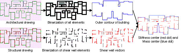
Figure B.1. Conversion of pixel shear wall elements to vectors