Semi-supervised learning method incorporating structural optimization for shear‑wall structure design using small and long-tailed datasets

1.       Introduction

Intelligent structural design is one of the key capabilities that can transform traditional construction industry practices into autonomous smart systems in the era of Construction 4.0 [1-3]. In recent years, machine learning (ML)-based intelligent structural design has progressed rapidly into a state that is potentially viable for practical applications [4]. In this paradigm, smart systems developers are not required to define or utilize specific design rules, as entailed by the traditional structural optimization methods. Instead, only the architecture of the ML algorithm needs to be defined and training data be provided for the algorithm to learn. The axiom is that the ML algorithm can automatically and implicitly discover effective design rules from the given input data [4]. However, since the design rules themselves are derived from data, the effectiveness of the current ML methods is therefore heavily dependent on the quality and quantity of the training data. The underlying data issues have become an important factor restricting the applications of the ML methods in practical structural design [5-6].

The present study attempts to solve two major problems inherent in intelligent structural design applications - namely, (1) data are typically available in insufficient amounts (Figure 1(a)) and (2) data are imbalanced with long-tailed distributions (Figure 1(b)). These issues are elaborated in what follows.

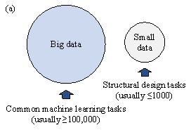
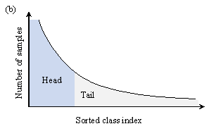
Figure 1. Data problems for structural design tasks. (a) Small data; (b) Long-tailed distribution.

Structural design tasks are generally formulated as supervised learning tasks, and the required data include inputs and labels. The inputs are typically architectural designs (e.g., floor layouts), which are relatively easy to obtain [7-8]; and design conditions (e.g., seismic and wind loads), which can be extracted from relevant codes and guidelines [9-10]. Note that different inputs can be obtained by combining an architectural design with different design conditions. The labels are typically high-level structural designs corresponding to the inputs (i.e., a combination of architectural design and design conditions), and are difficult and expensive to obtain because of intellectual property, confidentiality, and other concerns.

Therefore, in reality, developers usually have access to only a small amount of labeled data (i.e., data with architectural designs, design conditions, and the corresponding high-level structural designs) and a large amount of unlabeled data (i.e., data with only architectural designs and design conditions). This type of problem can, however, be effectively solved using semi-supervised learning methods [11]. Amongst various options, self-training is a classic method showing good versatility, simple implementation, and notable effectiveness [12-13]. The basic process of self-training is as follows: an ML model is first trained on labeled data, then the unlabeled data are annotated with proxy labels using the trained model and are added to the training set, and finally, the ML model is re-trained on the enlarged training set. Inspired by this process, we herein propose to formulate a schematic structural design task as a semi-supervised learning problem to address the issue of insufficient labeled data.

Besides suffering from being insufficient, real-world datasets often exhibit long-tailed distribution, where a small portion of classes (i.e., “head” classes) have a large number of data points, whereas the rest (i.e., “tail” classes) have few data points [14], as illustrated in Figure 1(b). For structural design tasks, this means that most structural design data are associated with only a few design conditions [15]. ML models trained on long-tailed datasets tend to be biased towards the head classes, resulting in poor performance on the tail classes. Therefore, the models may fail to provide rational structural designs under tail design conditions. Since self-training cannot improve the long-tailed data distribution pattern, it cannot be directly applied to the semi-supervised learning of long-tailed datasets [14]. Existing variants of self-training for long-tailed learning are limited to classification tasks [16-18]. It is difficult to apply them to regression tasks, which tends to be the case for structural design tasks.

To solve these data problems commonly encountered in intelligent structural design, this study proposes to incorporate a structural optimization method into a self-training framework. The proxy labels (i.e., structural designs) generated by the biased model are optimized to improve the data distribution characteristics, thereby obtaining a balanced dataset. On this basis, a standard self-training process is performed to further enlarge the dataset. The proposed method is expected to address the insufficient data and long-tailed data distribution issues simultaneously. Note that the proposed method is applicable to various structural design tasks for which a large number of unlabeled data are readily obtainable by combining architectural designs with different design conditions.

It is worth mentioning that the existing structural optimization methods have certain limitations, requiring developers to define all design rules artificially and hard-code them into the algorithm through objective functions, constraints, variable ranges, and so forth. [19-20]. In complex real-world problems, it is often difficult to comprehensively define the design rules and ensure that the algorithm can obtain a feasible solution within an acceptable time, which limits the applications of the existing structural design methods based solely on optimization methods. Therefore, this study uniquely combines the ML-based intelligent structural design methods [15, 21-23] with structural optimization methods [24-26], which not only breaks through the latter's limitations caused by artificially-defined design rules, but also alleviates the former’s dependency on data quality and quantity.

To validate its feasibility, the proposed method is applied to the schematic design of shear‑wall structures, which are widely used to build high-rise residential buildings as lateral load resisting systems for seismic events. A rational shear-wall layout can provide sufficient horizontal and vertical bearing capacities with low material consumption. In the schematic design phase for a shear-wall structure, structural engineers must propose a planar layout of the shear walls based on their experience and provide a basis for subsequent detailed design phases. They need to repeatedly adjust the structural design to satisfy the requirements of architects and contractors in a limited time. Therefore, design efficiency is highly valued in this preliminary design phase. Note that the shear-wall layout task does not have an explicit engineering function, as the engineer’s understanding of design requirements and constraints is still inaccurate and insufficient at this initial stage. It is also a time-consuming task for numerical simulation, as a large number of shell elements are required for finite element analysis, resulting in a high calculation complexity. Hence, it is necessary and suitable to use an appropriate ML method to perform this task. Existing research has proposed intelligent structural design methods for shear-wall structures based on deep learning technologies such as generative adversarial networks [15, 21-23]. However, these approaches all involve supervised learning based on large-scale datasets, and their applicability to small, long-tailed datasets remains unclear. Several researchers have also proposed structural optimization methods for shear-wall layout based on heuristic algorithms, such as genetic algorithm, tabu search, etc. [24-26]. However, the integration of these structural optimization methods into a semi-supervised learning framework has yet to be studied.

In summary, this study proposes a semi-supervised learning method in conjunction with structural optimization to solve the data problems commonly encountered in intelligent structural designs. The proposed method is then applied to the schematic design of shear‑wall structures. The remainder of this paper is organized as follows. Section 2 summarizes related prior studies. Section 3 presents the proposed semi-supervised learning method and a shear‑wall layout optimization procedure based on a two-stage evaluation strategy and the previously established empirical design rules. Section 4 describes the numerical experiments conducted using the proposed approach and its comparison with the existing methods. Section 5 presents a case study of a typical shear‑wall structure designed using different methods and evaluated in terms of code compliance, material consumption, and design efficiency. Finally, Section 6 outlines the conclusions of this study.

2.       Related research

2.1 Machine learning-based intelligent structural design methods

ML-based intelligent structural design methods have recently made remarkable progress in various practical tasks, including optimized shape, topology, and sizing design. ML algorithms adopted in related research include convolutional neural networks [27-28], generative adversarial networks (GANs) [21, 29], variational autoencoders [30-31], and graph neural networks [32], etc. Amongst these algorithms, GAN-based methods have made significant breakthroughs in the schematic design of shear‑wall structures [15, 22-23], and will be adopted in this study.

Unlike traditional structural optimization methods, ML-based intelligent structural design methods do not require artificially-defined design rules. Instead, they can automatically discover the rules from the training data. In addition, such methods can complete a structural design in seconds once training is complete, which has significant efficiency advantages compared to the conventional structural optimization methods that typically require hours of running time. However, previously mentioned difficulties in obtaining labeled (structural design) data have become a major challenge in this particular thread of studies [4-6].

2.2 Semi-supervised learning

Semi-supervised learning is a branch of ML that aims to solve problems using both labeled and unlabeled data [11]. Like many other application scenarios, a large amount of unlabeled data and a small amount of labeled data can be obtained in typical structural design tasks. By using these unlabeled data, semi-supervised learning is expected to exceed the design performance when using labeled data only.

Self-training is a classic semi-supervised learning method originally used in classification tasks. A classifier is first trained on a small-scale labeled dataset, then used to annotate unlabeled data with proxy labels, and is finally re-trained on the enlarged labeled dataset [12]. This method can also be applied to more general regression tasks [33]. Self-training can be employed to complete various structural design tasks while being simple to implement and effective [12]. It is worthwhile noting that the basic assumption of self-training is that the predictions of the trained model are deemed to be accurate [34]. However, this assumption does not hold true when the labeled dataset follows a long-tailed data distribution because the model will be biased toward generating proxy labels of head classes. Therefore, the application of self-training to long-tailed labeled datasets requires further study.

2.3 Long-tailed learning

In real-world problems, the collected training data usually follow a long-tailed distribution ‒ i.e., a small number of classes have massive data points, whereas the remaining classes have only a few data points [14]. The distribution of structural design data on design conditions also follows a similar pattern [15]. Long-tailed learning aims to train models that perform well across all classes using datasets with long-tailed distributions. Although self-training cannot be directly used to handle long-tailed data problems, some variants have been proposed to address these issues, such as CReST [17], DARS [18], and MosaicOS [19]. However, the scope of those methods is limited to classification tasks, whereas the present study focuses on more complex regression tasks in structural design.

2.4 Structural optimization methods

Structural optimization methods have been extensively studied over the past few decades. Existing studies can generally be categorized into gradient-based and heuristic methods [19-20]. Gradient-based methods find the optimal solution by solving the gradient, e.g., optimality criteria [35] and nonlinear programming [36]. Heuristic methods are usually inspired by natural phenomena and feature different ways of finding solutions in the design space. Methods in this latter category include genetic algorithms [24, 26], harmonic search [37-38], and particle swarm optimization [39]. The above two categories of methods differ in determining the optimal solution, but both require developers to artificially define all design rules by setting objective functions, constraints, variable ranges, etc. Structural design tasks in the real world often need to conform to very complex design rules and take into account numerous factors, making it difficult to design the optimization algorithm and obtain the solution in a quick manner. This results in limited applications of structural optimization methods in engineering practice. Given the above-mentioned technological challenges, this study will use the well-established genetic algorithm to improve the long-tailed data distribution, thereby enhancing the outcome of semi-supervised learning.

3.       Semi-supervised learning method incorporating structural optimization

The proposed semi-supervised learning method consists of six modules, as shown in Figure 2.

Module 1: First round of model training. An ML model Model-SL is trained on the collected small, long-tailed (SL) dataset. Owing to the unbalanced distribution of training data, the model is biased towards the head design conditions.

Module 2: First generation of proxy labels. Inputs are constructed corresponding to the tail design conditions, and their proxy labels are generated by Model-SL. These proxy-labeled data are used to complement the long-tailed dataset and balance its distribution. Since the proxy labels are generated by a biased model, they cannot entirely satisfy the specified tail design conditions.

Module 3: Optimization of proxy labels. The structural optimization method mentioned above is used to optimize the first-generation proxy labels, leading to rational structural designs under specified design conditions.

Module 4: Second round of model training. The optimized proxy-labeled data and the small, long-tailed dataset are merged into a small, balanced (SB) dataset. An ML model Model-SB is trained on this updated dataset, starting from the saved checkpoint of Model-SL. The bias of Model-SB is therefore reduced.

Module 5: Second generation of proxy labels. Inputs are constructed corresponding to all design conditions, and their proxy labels are generated by Model-SB, thereby further expanding the dataset.

Module 6: Third round of model training. The second-generation proxy-labeled data and the small, balanced dataset are merged into a large, balanced (LB) dataset. An ML model Model-LB is trained on the further updated dataset, starting from the saved checkpoint of Model-SB.

The proposed method is applicable to structural design tasks that can acquire a large amount of unlabeled data by combining architectural designs with different design conditions. In this study, this method is applied to the shear-wall layout task for validation. For the shear-wall layout task, the design variables include the positions and geometries of the shear walls. The design objective is to satisfy the structural requirements, such as limiting the inter-story drift under earthquakes, while minimizing the use of materials like concrete. To achieve this, an ML model updates its design variables in the form of pixel colors by mimicking labels (see Section 3.2). On the other hand, a structural optimization method updates its design variables in the form of wall lengths based on hard-coded rules (see Section 3.3). Note that the proposed design process is completely automatic and does not require any manual assignment.

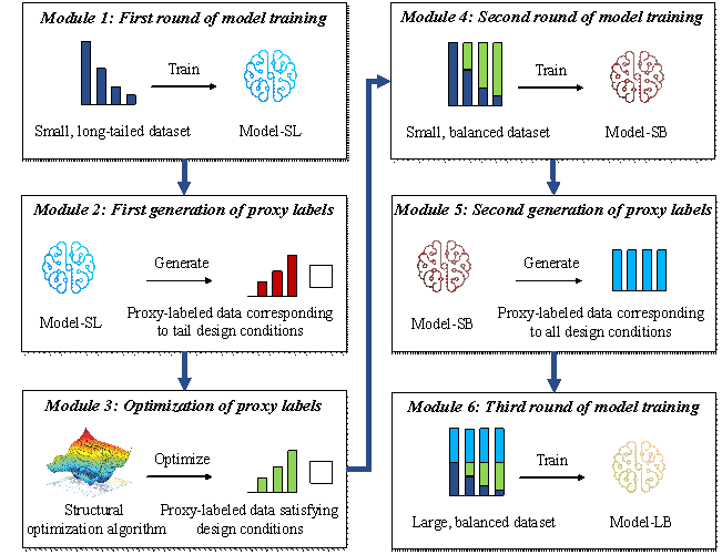
Figure 2. Proposed semi-supervised learning method incorporating structural optimization

3.1 Dataset

The dataset is established according to the key design conditions of the target structural design task. For the shear‑wall layout task, the horizontal and vertical load-bearing capacity requirements must be considered simultaneously. In the horizontal direction, seismic action is usually the dominant factor. Seismic action can be characterized by the seismic influential factor , which comprehensively reflects the seismic risk, site conditions, and structural dynamic characteristics [10, 40], as specified in Appendix A. Note that, the factor  is divided into four classes: S1 , S2 , S3 , and S4 . The key influencing factor in the vertical direction is the building height H, which is the distance from the roof to the ground [21-22]. The building height H is also divided into four classes: H1 , H2 , H3 , and H4 .

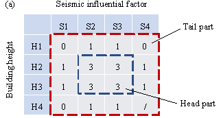
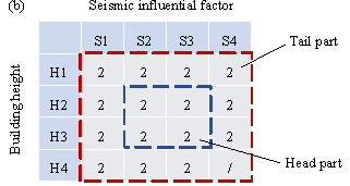
Figure 3. Distribution of data points on design conditions. (a) Long-tailed training set; (b) Balanced test set.

Considering the seismic influential factor and building height, a small, long-tailed training set (20 data points) and a balanced test set (30 data points) are constructed. The small, long-tailed training set has more data points (3 data points) on the four design condition combinations of S2 or S3 with H2 or H3, and few data points (0–1 data points) on other design condition combinations, thereby simulating a real-world long-tailed distribution, as illustrated in Figure 3(a). The design condition combinations with sufficient data points (≥ 3 data points) are called the head part; otherwise, they are called the tail part. The balanced test set has the same number of data points for all possible design condition combinations to test the generalization of the ML models under different scenarios, as demonstrated in Figure 3(b). It should be noted that according to the Chinese "Code for Seismic Design of Buildings" [10], it is fundamentally impossible for S4 and H4 to co-exist; therefore, the combination of S4 and H4 is not considered in the two datasets.

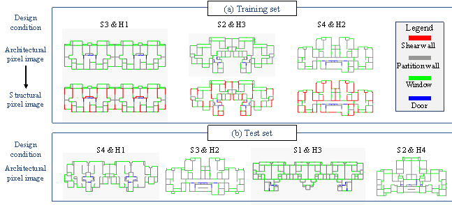
Figure 4. Typical semantic pixel images for different design conditions. (a) Training set; (b) Test set.

The required 50 sets of architectural and structural computer-aided design (CAD) drawings were collected from several leading architectural design institutes in China. These CAD drawings have been fully optimized by engineers for real-world engineering projects, satisfying all the code-specified requirements and demonstrating excellent cost-effectiveness. They are superior to the "optimal designs" obtained through structural optimization algorithms, which usually consider limited code-specific requirements and may not be feasible for real-world projects. Therefore, the collected design data are of high quality and best suited for training the ML models.

To facilitate the ML model to extract key features and avoid the interference of irrelevant information, architectural and structural designs are represented in the form of semantic pixel images [21]. Specifically, the coordinates of four key components (i.e., shear wall, partition wall, window, and door) are extracted from the CAD drawings, and the four key components are represented as red (RGB = (255, 0, 0)), gray (RGB = (132, 132, 132)), green (RGB = (0, 255, 0)), and blue (RGB = (0, 0, 255)) rectangles, respectively [23]. Typical semantic pixel images and the corresponding design conditions are presented in Figure 4, where the structural pixel images of the test set are not visible to the ML models. Finally, data augmentation (horizontal and vertical flipping) is used to enlarge the datasets fourfold.

3.2 Intelligent structural design based on generative adversarial networks

StructGAN-TXT is adopted to simultaneously consider the influence of architectural pixel images and design‑condition texts on the generation of structural pixel images [22]. The architecture of StructGAN-TXT is shown in Figure 5, including a generator and discriminator. The input of the model is the architectural pixel image and design conditions, and the output is the structural pixel image. The generator performs feature extraction and fusion of architectural pixel images and design‑condition texts and generates realistic structural pixel images based on the fused features to fool the discriminator. The discriminator judges whether the given structural pixel image is real or fake, attempting to accurately identify the structural pixel images generated by the generator. After a zero-sum game between the generator and discriminator, they finally reach a Nash equilibrium. Through this process, the generator learns the probability distribution of the labels based on the inputs, and the discriminator can no longer distinguish the generated labels from the real ones.

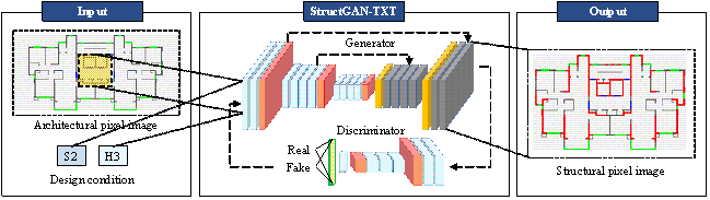
Figure 5. Architecture of StructGAN-TXT (Modified from [22])

The loss functions of the generator and discriminator are given in Equations (1) and (2), respectively [22]. During the model training, they are minimized by the optimizer.

where  and  are the conditional GAN losses of the generator and discriminator, respectively;  and  are the losses of the generated features and VGG19 [41] extracted features, respectively;  is the weight of feature loss;  and  are the text losses of the generator and discriminator, respectively, as shown in Equations (3) and (4);  and  are the weights of the text losses of the generator and discriminator, respectively.

where  is the cosine similarity function;  and  are the feature vectors of the real and fake texts, respectively;  is the feature vector of the real image;  is the binary cross-entropy loss function.

The dataset is collected as described in Section 3.1, and the key parameters used in the experiment are given in Section 4.1. After the training, the model is evaluated using the metrics given in Section 4.2. More details can be referred to [22].

Note that StructGAN-TXT is effective for the shear-wall layout task concerned in this study. For other design tasks, appropriate ML models should be selected considering the specific characteristics of the given problems.

3.3 Structural optimization based on a two-stage evaluation strategy and empirical design rules

To optimize the proxy labels (i.e., Module 3 in Figure 2), a shear-wall layout optimization procedure is developed based on a two-stage evaluation strategy and the previously established empirical design rules, as shown in Figure 6. The optimization variables are the shear-wall lengths (see step ③ below) and the optimization objective is to satisfy the structural requirements (i.e., inter-story drift under earthquakes) whilst consuming the minimum amount of materials (i.e., concrete). This optimization procedure is compatible with the input and output of StructGAN-TXT, enabling the automatic and efficient optimization of shear‑wall layouts. The detailed step-by-step procedure is described as follows.

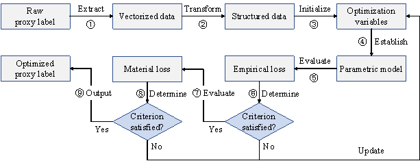
Figure 6. Structural optimization based on a two-stage evaluation strategy and empirical design rules

①     Extract vectorized data

The raw proxy labels generated by StructGAN-TXT are structural pixel images, where the shear walls are represented by red (RGB = (255, 0, 0)) pixels. The planar coordinates of the shear walls are obtained using a shear-wall extraction method based on computer vision and building information [23]. Firstly, the red pixels are stripped and binarized, and the noises are removed. Then, the endpoints of shear walls are identified as the intersection points between the axis of the partition wall and the contour of the shear-wall pixels.

②     Establish structured data

The structured data are established based on the planar coordinates of key components, as shown in Figure 7. The first level of structured data comprises architectural components, including partition walls, doors, and windows. The second level comprises nodes, including the endpoints of partition walls, doors, and windows, and the intersection nodes of partition walls in the X and Y directions. The third level comprises the node coordinates and shear-wall lengths on both sides of the intersection nodes. The shear-wall lengths are defined according to the coordinates obtained in step ①. A shear wall is moved to the nearest intersection node if it does not run over any intersection nodes.

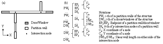
Figure 7. Illustration of the structured data. (a) Intersection node; (b) Relationship of three levels.

It can be found that these structured data allow the shear walls to be automatically grouped into local patterns in the form of "L", "T", and "X" shapes based on the locations of the intersection nodes, as shown in Figure 8. Two shear walls in the orthogonal directions that make up the local pattern will deform together, which is beneficial to the overall structural performance of the shear-wall structure. Furthermore, the local patterns can facilitate construction and reduce formwork costs, thereby improving constructability.

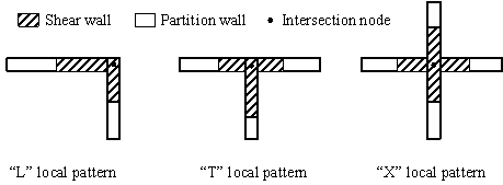
Figure 8. Local patterns of shear-wall layout

③     Initialize optimization variables

Based on the structured data, the shear-wall lengths on both sides of the intersection nodes are defined as the optimization variables. The lower bound (minimum value) of the variables is 0. The upper bound (maximum value) is (i) the distance from the intersection node to the endpoint of the partition wall or (ii) the distance from the intersection node to the midpoint of two intersection nodes, as shown in Figure 9(a). The increment of the variables should be defined according to the accuracy requirements, which can generally be taken as 250 mm. The initial value of the variables is defined according to the current shear-wall length.

There are three ways to reduce the possible combinations of variables, thereby accelerating convergence:

(1) Consider symmetry: In most cases, shear-wall structures of residential buildings are symmetrical along either the X or Y direction, as illustrated in Figure 4. If two intersection nodes are symmetrical along the X or Y direction and their variable bounds are identical, then the variables are shared by the two nodes. Note that the variables will not be merged for asymmetrical cases.

(2) Consider the optimization potential: Based on the initial value, a variable can be increased by  at most, and be decreased by no more than , as demonstrated in Figure 9(b). Therefore, the maximum change in the shear-wall length is . When , it is considered the shear wall exhibits a small optimization potential, and adjusting this shear wall has little effect on the structural performance of the overall structure. Therefore, this variable is frozen and not updated during the optimization process. Empirically, the threshold can be taken as 1000 mm.

(3) Consider the optimization tendency: Because StructGAN-TXT is trained on a long-tailed dataset, the proxy label generated on the new design conditions (tail part) will be biased towards the original design conditions (head part). If the optimization tendency can be determined, the variable bounds can then be further narrowed, as shown in Figure 9(c). Specifically, if all the new design conditions are either relaxed or unchanged, the shear-wall length should be reduced. Hence the bounds can be adjusted to [0, Initial value]; on the other hand, if all the new design conditions are either tightened or unchanged, the shear-wall length should be increased. Thus, the bounds are adjusted to [Initial value, Max value].

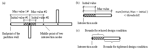
Figure 9. Optimization variable. (a) Variable bounds; (b) Optimization potential; (c) Optimization tendency.

After the optimization variables are initialized or updated, the shear-wall lengths should be checked to eliminate the presence of short-limb shear-walls [48]. Specifically, the length-to-thickness ratio  is defined as the ratio of wall length to wall thickness. If , the shear-wall length is extended to ensure that . If , the shear wall is removed.

④     Establish parametric model

Based on the optimization variables and structured data, a parametric model of the shear-wall structure can be established, including:

(1) Shear-wall layout: The planar coordinates of shear walls are obtained according to the current values of the optimization variables.

(2) Beam layout: First, beams are placed at all partition walls, doors, and windows, except where the shear walls have already been positioned. Topologically identified cantilever beams can then be adjusted not to appear by increasing or reducing the beam length. Finally, the empirical design rules proposed by Zhao et al. [42] are used to partition the coupling beams and the frame beams. Note that the beam layout strategy used in this study follows a simplified approach, which warrants further investigation. For instance, an upper limit for the beam span should be established to address concerns regarding gravity-load strength and serviceability design.

(3) Slab layout: Slabs are placed in all enclosed areas surrounded by shear walls and beams.

(4) Section size estimation: The thicknesses of shear walls are determined using the empirical design rules proposed by Lu et al. [15]. The heights of the frame and coupling beams are determined using the empirical design rules proposed by Zhao et al. [42]. The widths of the beams are the same as those of the shear walls.

⑤     First-stage evaluation based on empirical design rules

A quick evaluation of the shear-wall layout based on the following three empirical design rules:

(1) The shear-wall ratio should be within a reasonable range. The corresponding loss function can be calculated according to Equations (5)–(7). Empirically, when , this rule is satisfied.

where  is the shear‑wall ratio;  is the empirical optimal shear-wall ratio and can be obtained from Table 1, which is from the statistical data of a leading real-estate company in China;  is the cross-section area of all shear walls;  is the total floor area;  is the shear-wall length;  is the shear-wall thickness.

Table 1. Empirical optimal shear‑wall ratio

* 10% exceedance in 50 years; ** Building height

(2) The torsional radius of the shear walls should be larger than the radius of the gyration of the floor mass [43]. The corresponding loss function can be calculated using Equations (8)–(11) [24]. This rule is satisfied when  and .

where  is the distance between the geometric center of the shear wall i and the stiffness center of the structure;  and  are the lengths of the shear wall i in the X and Y directions, respectively;  is the polar moment of inertia of the floor mass in plan with respect to the center of mass of the floor;  is the floor mass.

(3) The shear walls should be able to support the floor load. The corresponding loss function is given in Equation (12). Empirically, when , this rule is satisfied.

where  is the floor area supported by the shear walls, which is obtained by estimating the floor area supported by each shear wall and then taking their union. Further details can be found in [24].

Finally, the total empirical loss is formulated as Equation (13).

where , , and  are the weighting factors of the three empirical design rules. Normally, .

⑥     Determine if the first-stage optimization is to be performed

If all the three empirical design rules in step ⑤ are satisfied, or the iteration number of optimization exceeds a preset threshold, then proceed to step ⑦ for finite‑element analysis.

Otherwise, an optimizer is deployed and the variables are updated. The optimizer adopts a genetic algorithm NSGA II [44]. The objective function  is to be minimized with no constraints.

⑦     Second-stage evaluation based on finite‑element analysis

A high-fidelity finite‑element model of the shear-wall structure is established. Shell elements are used to simulate the shear walls and the coupling beams, beam elements to simulate the frame beams, and membrane elements to simulate the slabs [45]. According to seismic design conditions, the response spectrum analysis of the model is performed under design earthquake loads. The maximum inter-story drifts in the X and Y directions (i.e.,  and ) are thus obtained.

The material loss (i.e., total concrete consumption) of the shear‑wall structure is also calculated, using Equation (14).

where , , , and  represent the concrete consumptions of shear walls, coupling beams, frame beams, and slabs, respectively.

For the schematic design of shear-wall structures, it is generally acceptable to only include concrete consumption in the material loss estimation [24-26]. For design tasks where steel reinforcement is essential to be considered, their material loss can be easily modified to include the reinforcement component, using the high-fidelity finite element model for calculation.

⑧     Determine if the second-stage optimization is to be performed

The optimizer updates the variables if the iteration number of optimization is smaller than a preset threshold. The optimization algorithm NSGA II [44] is also used herein. Leveraging non-dominated sorting, NSGA II can either solve multiple-objective problems by defining the Pareto domination relationship or solve constrained single-objective problems by defining the constrained domination relationship. The objective function  is to be minimized, and the constraints are set according to Equations (15)–(16).

where  and  are the maximum inter-story drifts in the X and Y directions, respectively;  is the inter-story drift limit under design earthquake loads [10].

Note that for the shear-wall layout task in the schematic design stage, only key metrics need to be considered. Therefore, the inter-story drifts under design earthquake loads are selected as the key constraints. Other load cases and constraints are, therefore, not considered in this study.

⑨     Output optimized proxy labels

Based on the structured data and the current optimum values of the variables, the coordinates of the shear walls, partition walls, doors, and windows are obtained to output a semantic pixel image. This pixel image can be directly used as a proxy label for training StructGAN-TXT.

4.       Numerical experiment

Numerical experiments are performed on a Windows computer with an NVIDIA GeForce RTX 3090 GPU and Intel Core i7-10700K CPU @ 3.80GHz. StructGAN-TXT is implemented in the PyTorch deep‑learning framework and is trained using the GPU. Through secondary development, the proposed structural optimization procedure is implemented via the parametric design software YJK-GAMA [46].

4.1 Step-by-step implementation

Module 1: First round of model training

StructGAN-TXT is trained using the hyperparameters provided in [22], as listed in Table 2. GAN is an advanced network architecture with strong image generation capability. Larger input and output sizes are adopted to generate high-resolution images, ensuring a high-fidelity ML model. The first round of training utilizes a small, long-tailed training set (Dataset-SL), and the trained model is Model-SL.

Table 2. Hyperparameters of StructGAN-TXT

Module 2: First generation of proxy labels

The first-generation proxy labels are used to form a balanced dataset, and therefore, should correspond to tail design‑condition combinations. For a given tail design‑condition combination, the seismic influential factor and the building height of the proxy label are randomly selected within its design‑condition class. Then, the architectural designs of the proxy labels are shared with the adjacent design‑condition combinations. A typical case is illustrated in Figure 10(a). Finally, 25 sets of inputs (i.e., architectural design and design conditions) are constructed, and the corresponding proxy labels are generated using Model-SL. Since Model-SL is biased, the above proxy labels are biased towards their original design conditions and cannot fully satisfy the new design conditions.

Note that if additional architectural designs are available, they can be used directly without adopting the sharing strategy shown in Figure 10(a). Otherwise, when choosing adjacent design condition combinations, it is preferable that the optimization tendency can be determined so that the variable bounds can be narrowed to accelerate convergence, as specified in Section 3.3, Step ③. When generating proxy labels, the combination of S4 and H4 is not considered, as it is not possible for them to coexist [10].

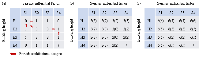
Figure 10. Distribution of proxy-labeled data. (a) Sharing of architectural designs; (b) Small, balanced dataset; (c) Large, balanced dataset (in parentheses are the numbers of proxy-labeled data)

Module 3: Optimization of proxy labels

The generated proxy labels are optimized using the proposed structural optimization procedure. For the genetic algorithm, an iteration number of 20 and a population size of 10 are used so that the time consumption is acceptable. Notably, the proposed structural optimization procedure can obtain satisfactory results with a smaller iteration number and population size than the conventional method by incorporating a two-stage evaluation strategy and empirical design rules. Other parameters are set as follows: the crossover probability is 0.9, the distribution index is 20 for both crossover and mutation operators, and the mutation probability is the inverse of the number of variables [44]. Depending on the complexity of the shear‑wall structures, the time consumption for each design varies from 1 h to 12 h. The optimization results are listed in Table 3, which are in line with expectations: the total length of the shear walls decreases in cases where the design conditions are either relaxed or unchanged, or increases in cases where the design conditions are either tightened or unchanged. For the cases where one design condition is relaxed and the other tightened, the change in the total shear‑wall length is minor. Note that the “Undetermined” class in optimization tendency should be minimized.

Table 3 also lists the number of variables before and after adopting the reduction strategy proposed in Section 3.3, Step ③. On average, the number of variables is reduced by 81% after considering three ways to decrease the possible combinations of variables.

Table 3. Optimization results and variable numbers of proxy labels

Figure 11 shows a comparison of proxy labels before and after optimization. The original design condition of this proxy label is S3H3, and the new design condition is S3H4. Since Model-SL is biased, it fails to generate sufficient shear walls under S3H4, and the resulting design is similar to that under S3H3, as shown in Figure 11(a). After optimization, the total shear‑wall length is significantly increased, which conforms better with the new design condition, as shown in Figure 11(b).

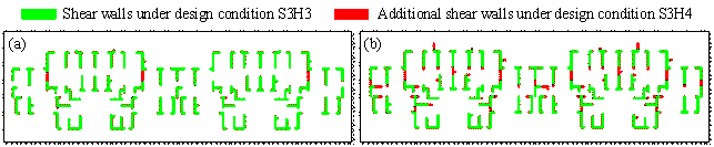
Figure 11. Comparison of proxy labels. (a) Before optimization; (b) After optimization.

Module 4: Second round of model training

The optimized proxy-labeled data are added into Dataset-SL to form Dataset-SB (Small, Balanced), whose data distribution is shown in Figure 10(b). Model-SB is trained on Dataset-SB from the checkpoint of Model-SL using the hyperparameters given in Table 2.

For comparison, Dataset-SB-F (Small, Balanced, Fake) is constructed based on the traditional self-training. Its data distribution is consistent with Dataset-SB (Figure 10(b)), but its proxy labels are directly generated by Model-SL without performing structural optimization. Similarly, Model-SB-F is trained on Dataset-SB-F from the checkpoint of Model-SL using the hyperparameters given in Table 2.

Module 5: Second generation of proxy labels

The second-generation proxy labels are used to further expand the small, balanced dataset, covering all design-condition combinations. Forty-five sets of inputs are constructed in total (i.e., three inputs for each design‑condition combination), and the corresponding proxy labels are generated using Model-SB.

Module 6: Third round of model training

The second-generation proxy-labeled data are added into Dataset-SB to form Dataset-LB (Large, Balanced), whose data distribution is shown in Figure 10(c). Model-LB is trained on Dataset-LB from the checkpoint of Model-SB using the hyperparameters given in Table 2.

For comparison, Dataset-LB-F (Large, Balanced, Fake) is constructed based on the traditional self-training. Its data distribution is consistent with Dataset-LB (Figure 10(b)), but its proxy labels are generated by Model-SL instead of Model-SB. Model-LB-F is trained on Dataset-LB-F from the checkpoint of Model-SL using the hyperparameters given in Table 2.

A typical training curve for the above-mentioned three rounds of model training is shown in Figure 12. Since the training set keeps increasing, the number of iterations in the three training rounds increases sequentially, which takes approximately 1h, 2h, and 4h training time, respectively.

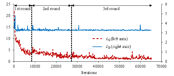
Figure 12. Typical training curve

4.2 Evaluation metrics

StructGAN-TXT models are tested on the balanced test set. The following metrics are used to evaluate the design performance [23].

where  and  are the total shear-wall lengths in the X and Y directions, respectively, designed by StructGAN-TXT;  and  are the total shear-wall lengths in the X and Y directions, respectively, designed by engineers;  and  are, respectively, the intersection and union areas of the shear walls designed by StructGAN-TXT and engineers.

The metrics mentioned above are specially designed for the shear-wall layout task. Among them,  reflects the similarity in the shear‑wall distribution,  reflects the similarity in the shear‑wall lateral stiffness, and  reflects the overall similarity. Note that structural design is a creative work without a standard answer. A structural design is acceptable as long as it satisfies the structural performance and other code-specified requirements. The design by StructGAN-TXT can be different from that by engineers, which does not necessarily mean that the former is unreasonable. Therefore, the design performance of StructGAN-TXT cannot be properly evaluated with  alone.  is a more reasonable evaluation metric that considers the similarity of the structural performance in terms of the shear‑wall lateral stiffness. According to our previous research [21, 23], a design result is considered acceptable if . However, a value of  does not guarantee a perfect structural design. As such, further exploration is needed in the evaluation metrics of ML-generated structural design.

Meanwhile, the following metric is used to measure the performance difference between the head and tail design conditions.

where  and  are the averaged  on the head and tail design conditions, respectively.

4.3 Results of experiment

The five models described in Section 4.1 are experimentally compared. Model-SL, Model-SB, and Model-LB are the results of the first, second, and third round of model training shown in Figure 2, respectively. Model-SB-F and Model-LB-F are the control groups that use the traditional self-training.

Three independent experiments are performed on the five models, and their design performances ( ) on the test set are shown in Figure 13. Compared with Model-SL, Model-SB improves the performance on the tail and head design conditions by 9.1% and 4.6%, respectively. This suggests that the proposed method can improve the design performance for all classes. Model-LB improves the performance on the tail and head design conditions by 11.6% and 4.3%, respectively. Its performance on all design conditions is better than the outcome of Model-SB. This implies that further enlarging the small, balanced dataset is effective. For comparison, Model-SB-F yields an improvement of 3.9% in both tail and head design conditions, and Model-LB-F makes an improvement of 0.9% and 2.8%, respectively, in the tail and head design conditions. These results indicate that the traditional self-training is much less effective in improving the design performance on the tail design conditions.

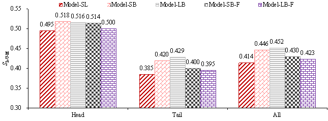
Figure 13. Design performance ( ) of five models (average of 3 independent experiments)

The performance differences ( ) between the head and tail design conditions of the five models on the test set are shown in Figure 14. Compared with Model-SL,  of Model-SB is reduced by 10.6%, which is better than Model-SB-F, which yields a 3.7% increase;  of Model-LB is reduced by 21.3%, which is also better than that of Model-LB-F, which is 5.6%. Therefore, compared with the traditional self-training, the proposed method can better reduce the performance differences between the head and tail design conditions.

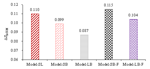
Figure 14. Performance difference ( ) of five models (average of 3 independent experiments)

4.4 Comparison with direct method

It is worthwhile recognizing that, the structural optimization method proposed in Section 3.3 can be used directly to improve the quality and quantity of the training data. However, compared to the direct method, the proposed semi-supervised learning method is superior in efficiency and more conducive to solving data problems in practical design projects.

Specifically, (1) Dataset-SL has 20 data points, and Dataset-LB has 90 data points. If the direct method is adopted, 70 data points would need to be optimized by the genetic algorithm. In contrast, only 25 data points need to be optimized if the proposed method is used. (2) The direct method takes the original design as a starting point for optimization, whereas the proposed method starts from the preliminary design given by GAN, which is much closer to an ideal design. Therefore, the proposed method is expected to obtain an optimized design solution faster and better.

5.       Case study

5.1 Basic information

A typical shear-wall structure of a residential building is selected for the case study. The building has 30 stories and a total height of 86.8 m. As such, the height design condition is H4. The seismic intensity is 8 degrees, corresponding to a 0.20 g peak ground acceleration with an exceedance probability of 10% in 50 years. The seismic design group is Group 1, the site class is Class III, and the site characteristic period is 0.45 s. The seismic influential factor a is calculated as 0.309. Hence, the seismic design condition is S3. The building can be clearly identified as a tail design‑condition combination (Figure 3). Its architectural pixel image and structural pixel image designed by engineers are displayed in Figure 15.

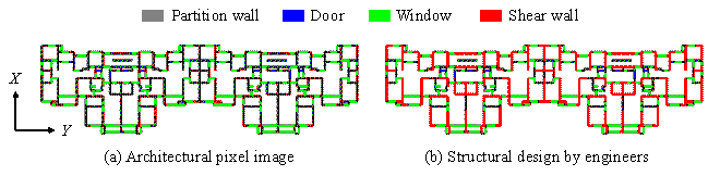
Figure 15. Typical shear‑wall structure of a residential building

5.2 Evaluation results

The building is individually designed using Model-SL and Model-LB, and their design outcomes are presented in Figure 16. Note that the shear walls are generated at the positions of partition walls and therefore will not influence the flexibility of the architectural layout. Additionally, the shear walls automatically form the local patterns as described in Section 3.3 and exhibit good constructability. Comparisons between the designs by the ML model and by engineers are shown in Figure 17. Because Model-SL is trained on the long-tailed dataset, its design does not have a sufficient arrangement of shear walls ( ), whereas that in Model-LB’s design is significantly increased ( ).

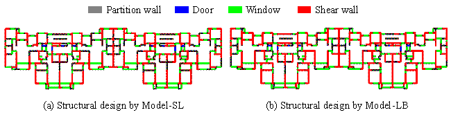
Figure 16. Design outcomes of Model-SL and Model-LB

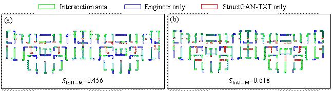
Figure 17. Design results of the typical case study. (a) Model-SL; (b) Model-LB.

Subsequently, finite‑element models corresponding to the three structural designs are established in the structural design software YJK [47] using the method described in Section 3.3. Response spectrum analyses are performed, and the maximum inter-story drifts are shown in Figure 18. Owing to the insufficient lateral stiffness of the Model-SL design, its inter-story drift in the X direction exceeds the code limit [10]. In contrast, the inter-story drifts of the Model-LB design can satisfy the code requirements and are closer to those of the engineer's design. Note that Y-direction shear-wall length design is not governed by the inter-story drift in the Y direction. Instead, it is determined by other factors, such as vertical loads and torsional radius, which are considered using empirical design rules specified in Section 3.3. Other code requirements, such as the bearing capacity of structural components, are usually checked in the detailed design phase and are therefore not discussed herein.

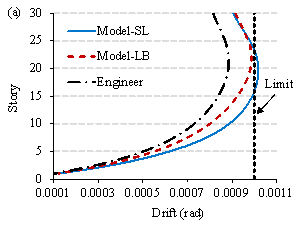
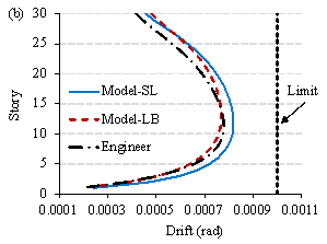
Figure 18. Inter-story drifts under design-level earthquakes. (a) X direction; (b) Y direction.

Table 4 summarizes the performance outcomes of different designers. Compared with Model-SL, Model-LB has better code compliance. Compared with engineers, Model-LB demonstrates a remarkably increased design efficiency and a slightly reduced concrete consumption. Specifically, the 30 hours spent by structural engineers include a 20-hour design task and a 10-hour modeling task. The 8 minutes consumed by the proposed method include 5 minutes of preprocessing, 1 minute of designing, and 2 minutes of modeling. Such design efficiency has been reported by consulting senior engineers [23].

Table 4. Summary of different designers’ outcomes

It is worth noting that the ML-based intelligent structural design can be completed in 8 minutes. However, the same task will take 1‒12 hours to complete when a structural optimization method is used. This can be very inconvenient for the preliminary, schematic design phase, during which a large number of proposals are designed and compared. It is important to note that the ML-based approach and the structural optimization method are fundamentally different, although both are computer-aided design techniques that can provide preliminary designs for engineers. The comparison made herein aims to demonstrate their respective efficiencies in performing preliminary designs for engineers to reference.

6.       Conclusions

This study proposes a semi-supervised learning method incorporating the structural optimization approach, aiming to solve the small‑data and long-tailed distribution problems that are typically encountered in ML-based intelligent structural design. The proposed method is applicable to structural design tasks that can acquire a large amount of unlabeled data with relative ease by uniquely combining architectural designs with different design conditions. In this method, first, a structural optimization method is incorporated into a self-training framework, which transforms the long-tailed distribution of the training data into a balanced one. Then, a standard self-training process is performed to further expand the training set. Additionally, a shear-wall layout optimization procedure is developed based on a two-stage evaluation strategy and the previously established empirical design rules, which enables automatic and efficient optimization of the proxy labels. Finally, the proposed method is applied to the schematic design of shear-wall structures. The following conclusions could be drawn from this study:

(1) The proposed semi-supervised learning method enables an effective application of the ML-based intelligent structural design methods to small, long-tailed datasets.

(2) The proposed structural optimization procedure is compatible with the input and output of GANs, facilitating an efficient optimization of the shear-wall layout, thereby automatically obtaining proxy labels that can satisfy the given design conditions.

(3) The application on the shear-wall layout task reveals that, compared with the conventional supervised learning method, the proposed method can improve the design performance on the tail design conditions by 11.6% and reduce the performance difference between the head and tail design conditions by 21.3%.

(4) The case study of a typical shear-wall structure discovers that, compared with the design by a conventional supervised learning method, the design by the proposed method satisfactorily resembles that by design engineers whilst meeting key code-specified requirements.

Henceforth, the applicability of the proposed method to other structural design tasks and the associated ML models merits additional confirmation. Moreover, other means of combining ML-based intelligent structural design methods with structural optimization methods necessitate further investigation. Lastly, the shear-wall layout optimization procedure should be enhanced to reduce the impact of premature convergence and the tendency to be trapped in local optima [49]. Additionally, it should incorporate further aspects of seismic design, such as axial and shear force responses under earthquakes.

Appendix A

The seismic influential factor  can be calculated using Equation (A1) [10].

where  is the maximum seismic influential factor, which can be determined according to Table A1;  is the site characteristic period (s), which can be found in Table A2;  is the basic natural period of the building structure, which can be calculated from Equation (A2) [9].

where  and b are the height and width of the building structure, respectively.

Table A1 Maximum seismic influential factor [10]

Table A2 Site characteristic period (s) [10]

Acknowledgment

References

[1]      Baduge SK, Thilakarathna S, Perera JS, Arashpour M, Sharafi P, Teodosio B, et al. Artificial intelligence and smart vision for building and construction 4.0: machine and deep learning methods and applications. Autom Constr 2022; 141: 104440. https://doi.org/10.1016/j.autcon.2022.104440

[2]      Forcael E, Ferrari I, Opazo-Vega A, Pulido-Arcas JA. Construction 4.0: a literature review. Sustainability 2020; 12(22): 9755. https://doi.org/10.3390/su12229755

[3]      Muñoz-La Rivera F, Mora-Serrano J, Valero I, Oñate E. Methodological-technological framework for Construction 4.0. Arch Comput Methods Eng 2021; 28(2): 689–711. https://doi.org/10.1007/s11831-020-09455-9

[4]      Málaga-Chuquitaype C. Machine learning in structural design: an opinionated review. Front Built Environ 2022; 8: 815717. https://doi.org/10.3389/fbuil.2022.815717

[5]      Akinosho TD, Oyedele LO, Bilal M, Ajayi AO, Delgado MD, Akinade OO, et al. Deep learning in the construction industry: a review of present status and future innovations. J Build Eng 2020; 32: 101827. https://doi.org/10.1016/j.jobe.2020.101827

[6]      Sun H, Burton HV, Huang H. Machine learning applications for building structural design and performance assessment: state-of-the-art review. J Build Eng 2021; 33: 101816. https://doi.org/10.1016/j.jobe.2020.101816

[7]      Nauata N, Hosseini S, Chang K-H, Chu H, Cheng C-Y, Furukawa Y. House-GAN++: generative adversarial layout refinement networks. In Proceedings of the IEEE/CVF Conference on Computer Vision and Pattern Recognition 2021. https://doi.org/10.1109/CVPR46437.2021.01342

[8]      Qian W, Xu Y, Li H. A self-sparse generative adversarial network for autonomous early-stage design of architectural sketches. Comput-Aided Civ Infrastruct Eng 2021; 37(5): 612-628. https://doi.org/10.1111/mice.12759

[9]      MOHURD. Load code for the design of building structures (GB50009-2012). Beijing: China Architecture & Building Press; 2012. (in Chinese)

[10]  MOHURD. Code for the seismic design of buildings (GB50011-2010). Beijing: China Architecture & Building Press; 2016. (in Chinese)

[11]  van Engelen JE, Hoos HH. A survey on semi-supervised learning. Mach Learn 2020; 109(2): 373–440. https://doi.org/10.1007/s10994-019-05855-6

[12]  Triguero I, García S, Herrera F. Self-labeled techniques for semi-supervised learning: taxonomy, software and empirical study. Knowl Inf Syst 2015; 42(2): 245–284. https://doi.org/10.1007/s10115-013-0706-y

[13]  Xu YJ, Lu XZ, Fei YF, Huang YL. Iterative self-transfer learning: a general methodology for response time-history prediction based on small dataset. J Comput Des Eng 2022; 9(5): 2089–2102. https://doi.org/10.1093/jcde/qwac098

[14]  Zhang Y, Kang B, Hooi B, Yan S, Feng J. Deep long-tailed learning: a survey. arXiv 2021. https://doi.org/10.48550/arXiv.2110.04596

[15]  Lu XZ, Liao WJ, Zhang Y, Huang YL. Intelligent structural design of shear wall residence using physics-enhanced generative adversarial networks. Earthq Eng Struct Dyn 2022; 51(7): 1657-1676. https://doi.org/10.1002/eqe.3632

[16]  He R, Yang J, Qi X. Re-distributing biased pseudo labels for semi-supervised semantic segmentation: a baseline investigation. In Proceedings of the IEEE/CVF International Conference on Computer Vision 2021; 6930–6940. https://doi.ieeecomputersociety.org/10.1109/ICCV48922.2021.00685

[17]  Wei C, Sohn K, Mellina C, Yuille A, Yang F. CReST: a class-rebalancing self-training framework for imbalanced semi-supervised learning. In Proceedings of the IEEE/CVF Conference on Computer Vision and Pattern Recognition 2021; 10857–10866. https://doi.org/10.1109/CVPR46437.2021.01071

[18]  Zhang C, Pan T-Y, Li Y, Hu H, Xuan D, Changpinyo S, et al. MosaicOS: a simple and effective use of object-centric images for long-tailed object detection. In Proceedings of the IEEE/CVF International Conference on Computer Vision 2021; 417–427. https://doi.org/10.1109/ICCV48922.2021.00047

[19]  Aldwaik M, Adeli H. Advances in optimization of highrise building structures. Struct Multidiscipl Optim 2014; 50(6): 899–919. https://doi.org/10.1007/s00158-014-1148-1

[20]  Afzal M, Liu Y, Cheng JCP, Gan VJL. Reinforced concrete structural design optimization: a critical review. J Clean Prod 2020; 260: 120623. https://doi.org/10.1016/j.jclepro.2020.120623

[21]  Liao WJ, Lu XZ, Huang YL, Zheng Z, Lin YQ. Automated structural design of shear wall residential buildings using generative adversarial networks. Autom Constr 2021; 132: 103931. https://doi.org/10.1016/j.autcon.2021.103931

[22]  Liao WJ, Huang YL, Zheng Z, Lu XZ. Intelligent generative structural design method for shear wall building based on “fused-text-image-to-image” generative adversarial networks. Expert Syst Appl 2022; 210: 118530. https://doi.org/10.1016/j.eswa.2022.118530

[23]  Fei YF, Liao WJ, Zhang S, Yin PF, Han B, Zhao PJ, et al. Integrated schematic design method for shear wall structures: a practical application of generative adversarial networks. Buildings 2022; 12(9): 1295. https://doi.org/10.3390/buildings12091295

[24]  Tafraout S, Bourahla N, Bourahla Y, Mebarki A. Automatic structural design of RC wall-slab buildings using a genetic algorithm with application in BIM environment. Autom Constr 2019; 106: 102901. https://doi.org/10.1016/j.autcon.2019.102901

[25]  Lou H, Gao B, Jin F, Wan Y, Wang Y. Shear wall layout optimization strategy for high-rise buildings based on conceptual design and data-driven tabu search. Comput Struct 2021; 250: 106546. https://doi.org/10.1016/j.compstruc.2021.106546

[26]  Zhou X, Wang L, Liu J, Cheng G, Chen D, Yu P. Automated structural design of shear wall structures based on modified genetic algorithm and prior knowledge. Autom Constr 2022; 139: 104318. https://doi.org/10.1016/j.autcon.2022.104318

[27]  Ampanavos S, Nourbakhsh M, Cheng CY. Structural design recommendations in the early design phase using machine learning. In Proceedings of Computer-Aided Architectural Design. Design Imperatives: The Future is Now 2022; 190–202. https://doi.org/10.1007/978-981-19-1280-1_12

[28]  Yu Y, Hur T, Jung J, Jang IG. Deep learning for determining a near-optimal topological design without any iteration. Struct Multidiscipl Optim 2019; 59(3): 787–799. https://doi.org/10.1007/s00158-018-2101-5

[29]  Pizarro PN, Massone LM, Rojas FR, Ruiz RO. Use of convolutional networks in the conceptual structural design of shear wall buildings layout. Eng Struct 2021; 239: 112311. https://doi.org/10.1016/j.engstruct.2021.112311

[30]  Danhaive R, Mueller CT. Design subspace learning: structural design space exploration using performance-conditioned generative modeling. Autom Constr 2021; 127: 103664. https://doi.org/10.1016/j.autcon.2021.103664

[31]  Mirra G, Pugnale A. Comparison between human-defined and AI-generated design spaces for the optimisation of shell structures. Structures 2021; 34: 2950–2961. https://doi.org/10.1016/j.istruc.2021.09.058

[32]  Chang KH, Cheng CY. Learning to simulate and design for structural engineering. In Proceedings of the International Conference on Machine Learning 2020; 1426–1436. https://proceedings.mlr.press/v119/chang20a.html

[33]  Kostopoulos G, Karlos S, Kotsiantis S, Ragos O. Semi-supervised regression: a recent review. J Intell Fuzzy Syst 2018; 35(2): 1483–1500. https://doi.org/10.3233/JIFS-169689

[34]  Yang X, Song Z, King I, Xu Z. A survey on deep semi-supervised learning. arXiv 2021. https://doi.org/10.48550/arXiv.2103.00550

[35]  Chan CM, Wang Q. Nonlinear stiffness design optimization of tall reinforced concrete buildings under service loads. J Struct Eng 2006; 132(6): 978–990. https://doi.org/10.1061/(ASCE)0733-9445(2006)132:6(978)

[36]  Guerra A, Newman AM, Leyffer S. Concrete structure design using mixed-integer nonlinear programming with complementarity constraints. SIAM J Optim 2011; 21(3): 833–863. https://doi.org/10.1137/090778286

[37]  Akin A, Saka MP. Harmony search algorithm based optimum detailed design of reinforced concrete plane frames subject to ACI 318-05 provisions. Comput Struct 2015; 147: 79–95. https://doi.org/10.1016/j.compstruc.2014.10.003

[38]  Boscardin JT, Yepes V, Kripka M. Optimization of reinforced concrete building frames with automated grouping of columns. Autom Constr 2019; 104: 331–340. https://doi.org/10.1016/j.autcon.2019.04.024

[39]  Gandomi AH, Kashani AR, Roke DA, Mousavi M. Optimization of retaining wall design using recent swarm intelligence techniques. Eng Struct 2015; 103: 72–84. https://doi.org/10.1016/j.engstruct.2015.08.034

[40]  Fei YF, Liao WJ, Huang YL, Lu XZ. Knowledge-enhanced generative adversarial networks for schematic design of framed tube structures. Autom Constr 2022; 144: 104619. https://doi.org/10.1016/j.autcon.2022.104619

[41]  Simonyan K, Zisserman A. Very deep convolutional networks for large-scale image recognition. In Proceedings of the International Conference on Learning Representations 2015. https://doi.org/10.48550/arXiv.1409.1556

[42]  Zhao PJ, Liao WJ, Xue HJ, Lu XZ. Intelligent design method for beam and slab of shear wall structure based on deep learning. J Build Eng 2022; 57: 104838. https://doi.org/10.1016/j.jobe.2022.104838

[43]  CEN. Eurocode 8: Design of structures for earthquake resistance-part 1: general rules, seismic actions and rules for buildings. Brussels: European Committee for Standardization; 2004.

[44]  Deb K, Pratap A, Agarwal S, Meyarivan T. A fast and elitist multiobjective genetic algorithm: NSGA-II. IEEE Trans Evol Comput 2002; 6(2): 182–197. https://doi.org/10.1109/4235.996017

[45]  Lu X, Lu XZ, Guan H, Ye LP. Collapse simulation of reinforced concrete high‐rise building induced by extreme earthquakes. Earthq Eng Struct Dyn 2013; 42(5): 705-723. https://doi.org/10.1002/eqe.2240

[46]  YJK-GAMA secondary development guide. 2023. https://gitee.com/NonStructure/yjk-gama-secondary-development/ Last accessed: 7 Feb 2023. (in Chinese)

[47]  YJK-A: building structure calculation software. 2023. https://www.yjk.cn/article/36/ Last accessed: 7 Feb 2023. (in Chinese)

[48]  MOHURD. Technical specification for concrete structures of tall building (JGJ 3-2010). Beijing: China Architecture & Building Press; 2010. (in Chinese)

[49]  Machairas V, Tsangrassoulis A, Axarli K. Algorithms for optimization of building design: A review. Renew Sust Energ; 2014, 31: 101-112. https://doi.org/10.1016/j.rser.2013.11.036