2. REGIONAL SCALE NONLINEAR THA OF BUILDINGS CONSIDERING SCI EFFECTS
2.1 Nonlinear MDOF model for buildings above the ground
Lu et al. [2017a] proposed that the nonlinear MDOF models can simulate the dynamic behavior of buildings with satisfactory accuracy and efficiency for regional seismic damage simulation. Therefore, the nonlinear MDOF models for buildings (including MDOF shear models and MDOF flexural-shear models as shown in Figures 1A and 1B) and the corresponding parameter determination method proposed by Lu et al. [2017a] and Xiong et al. [2016, 2017] are adopted in this work to perform the nonlinear THA of buildings on a regional scale.
In general, low- and multi-story buildings often exhibit shear deformation modes under earthquakes, while tall buildings will deform in flexure-shear modes. So the MDOF shear model will be used for the low- and multi-story buildings, and the MDOF flexural-shear model will be adopted to tall buildings. The masses of the buildings are concentrated on their corresponding stories, and the nonlinear behavior of the structure is represented by the nonlinear inter-story force-displacement relationships. Thus, the parameter determination of the inter-story force-displacement relationships will be very important for the rationality and accuracy of the simulation results, considering the limited available information for buildings on a regional scale.
Xiong et al. [2016, 2017] proposed a parameter determination and damage state determination method for the MDOF shear and flexural-shear models. In their work, trilinear backbone curves are adopted for the inter-story force-displacement relationships (shown in Figure 1C), and a single parameter pinching model proposed by Steelman et al. [2009] is adopted. Firstly, based on building inventory data (including height, area, story number and so forth), a simulated design procedure is conducted according to the corresponding design codes, and the fundamental period and the design point on the backbone curve can be obtained. Then, according to related statistics of extensive experimental and analytical results, the yield point, peak point and softening point on the backbone curve can be further obtained, which in turn will determine the shape of the backbone curve. Five damage states, ranging from none, slight, moderate, to extensive and complete damage, are considered in their work. The reliability of the proposed method is further validated by comparing simulation results with actual seismic response.
![Figure 1 (A) MDOF shear model; (B) MDOF flexural-shear model; and (C) Trilinear backbone curve adopted in MDOF model [Xiong et al. 2016, Xiong et al. 2017].](./2018-EESD-SCI_Effect.files/image001.jpg)

Figure 1 (A) MDOF shear model; (B) MDOF flexural-shear model; and (C) Trilinear backbone curve adopted in MDOF model [Xiong et al. 2016, Xiong et al. 2017].
2.2 SPEED for simulating the wave propagation in 3D site models
To conveniently simulate the SCI effects, an open source program, SPEED [Mazzieri et al. 2013], is adopted in this work. The program can simulate seismic wave propagation in three-dimensional visco-elastic heterogeneous media on both local and regional scales. Based on the discontinuous Galerkin spectral approximation, SPEED can handle non-matching grids in an efficient and versatile way, and has been successfully applied in many cases, such as Christchurch in New Zealand, Thessaloniki in Greece and so forth [Abraham et al. 2016, Mazzieri et al. 2013, Evangelista et al. 2017, Smerzini et al. 2017].
The governing equation adopted in SPEED has the following expression to describe the wave propagation in the soil domain [Mazzieri et al. 2013]:
![]() (1)
(1)
where ¦Ń is the density of the soil; u, ![]() , and
, and ![]() represent the displacement, velocity and acceleration filed of the soil,
respectively; ¦Î is the decay factor; ¦Ň(u) is the Cauchy
stress tensor; and f is the density of body forces. The explicit Newmark
method (¦Â = 0, ¦Ă = 0.5) is adopted for time integration in the
dynamic simulation.
represent the displacement, velocity and acceleration filed of the soil,
respectively; ¦Î is the decay factor; ¦Ň(u) is the Cauchy
stress tensor; and f is the density of body forces. The explicit Newmark
method (¦Â = 0, ¦Ă = 0.5) is adopted for time integration in the
dynamic simulation.
2.3 Numerical coupling scheme for simulating SCI effects
Figure 2 illustrates the numerical coupling scheme for simulating SCI effects. The numerical scheme consists of two main parts. In the first part, wave propagation in the soil domain is solved by using SPEED via Equation (1). In the second part, each building is modeled using the nonlinear MDOF model. To couple these two parts, in each time step, the base reaction forces from buildings are imposed to the soil domain, and the acceleration computed from the soil domain are set as base acceleration to buildings. The detailed computation procedure is illustrated in Figure 2 and shown as follows.
(a) Given the soil response and boundary condition at tn,
the soil response at tn+1 , ![]() , can be solved via Equation (1) by using explicit Newmark integration scheme
(¦Â = 0, ¦Ă = 0.5). The equation can be written in a matrix form
for the whole soil domain as follows:
, can be solved via Equation (1) by using explicit Newmark integration scheme
(¦Â = 0, ¦Ă = 0.5). The equation can be written in a matrix form
for the whole soil domain as follows:
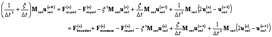 (2)
(2)
where the superscript represents the time step; the external load ![]() applied to the soil domain at tn consists of two different
sources:
applied to the soil domain at tn consists of two different
sources: ![]() represents boundary forces for seismic wave input at the bottom and wave
absorption at the sides of truncated soil domain, and
represents boundary forces for seismic wave input at the bottom and wave
absorption at the sides of truncated soil domain, and ![]() is the interaction force imposed to the soil domain at each building location,
which can be easily calculated as the base reaction force of the building from
dynamic structural analysis;
is the interaction force imposed to the soil domain at each building location,
which can be easily calculated as the base reaction force of the building from
dynamic structural analysis; ![]() denotes the internal load obtained from the soil response at tn;
Msoil is the mass matrix for the soil domain. Note that Equation
(2) has considered not only the soil-structure interaction at the building location,
but also propagation and interaction of wave field due to inconsistency of soil
motions at various locations, such that wave interaction among different building
locations, and wave interaction between the near field and the free field can
be naturally captured. It is also worth mentioning that heterogeneous soil layers
and complex 3D topography can also be modeled using the spectral element simulation
[Wang et al. 2018].
denotes the internal load obtained from the soil response at tn;
Msoil is the mass matrix for the soil domain. Note that Equation
(2) has considered not only the soil-structure interaction at the building location,
but also propagation and interaction of wave field due to inconsistency of soil
motions at various locations, such that wave interaction among different building
locations, and wave interaction between the near field and the free field can
be naturally captured. It is also worth mentioning that heterogeneous soil layers
and complex 3D topography can also be modeled using the spectral element simulation
[Wang et al. 2018].
(b) After obtaining the soil displacement field at tn+1,
the soil acceleration ![]() at each building location (e.g., A and B in Figure 2) at tn
can be assigned as base acceleration to each building using explicit Newmark
method as shown in Equation (3).
at each building location (e.g., A and B in Figure 2) at tn
can be assigned as base acceleration to each building using explicit Newmark
method as shown in Equation (3).
![]() (3)
(3)
(c) In this work, dynamic response analysis is performed individually
for each building using the nonlinear MDOF model shown in Figure 1. The nonlinear
structural responses of each building at tn+1,
![]() , can be obtained by solving Equation (4):
, can be obtained by solving Equation (4):
![]() (4)
(4)
where {1} stands for a vector of ones {1, 1, ˇ , 1}T;
Mbldg denotes the mass matrix of each building; Cbldg
represents matrix for Rayleigh damping; Fint,bldg denotes
the internal force obtained from the nonlinear building analysis. It is noted
that in solving the nonlinear structural responses, the base of each building
(e.g., A and B in Figure 2) is assumed to be fixed, and the base acceleration
![]() is imposed as inertia force to each story. Hence, the term ubldg
in Figure (2) and Equation (4) represents the buildingˇŻs displacement relative
to its base. As a result, the displacement compatibility at the building location
is implicitly satisfied.
is imposed as inertia force to each story. Hence, the term ubldg
in Figure (2) and Equation (4) represents the buildingˇŻs displacement relative
to its base. As a result, the displacement compatibility at the building location
is implicitly satisfied.
(d) Taken the base reaction force from each building at tn+1
as the updated interaction force, the updated ![]() is then applied to the soil domain at the building location for the next iteration.
is then applied to the soil domain at the building location for the next iteration.
(e) Loop over steps (a) to (d) until the last time step.
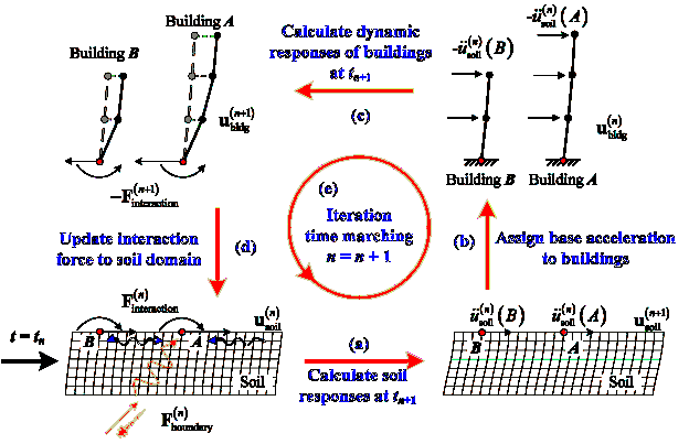
Figure 2 Numerical coupling scheme for SCI effects.
To implement the above procedure, first of all, the building inventory data are necessary. The building inventory data include the height, story number, structural type, year built, location of the building, and other design information. The vibration period of the building is optional. If this information is not provided, the vibration period of the building will be estimated based on empirical equations and the building inventory data. Secondly, to update the interaction force Finteraction to the soil domain, the corresponding Neumann boundary conditions should be assigned according to the location of each building. A new function type for boundary conditions has been developed in SPEED, so that the boundary force can be updated at each time step by using the value of Finteraction calculated from the MDOF models.
Compared with existing models that simulate the SCI effects, the numerical coupling scheme proposed in this work requires only the building inventory data and the updated force boundary as additional input. The backbone curves of the buildings can be calculated automatically within the program according to Xiong et al.ˇŻs work [Xiong et al. 2016, Xiong et al. 2017], which significantly reduces the workload of numerical modeling. The MDOF model can capture the nonlinear seismic response of buildings, which cannot be achieved if an elastic block model is used [Kato and Wang 2017]. Owing to the reduced DOFs, the adoption of MDOF models for buildings is highly cost-effective for the simulation. The proposed method can not only consider the SSI at the building locations due to the coupling scheme, but also the SSSI and SCI effects, since they have been naturally captured during the dynamic soil response simulation in SPEED.