A nonlinear computational model for regional seismic simulation of tall buildings

Chen Xiong, Xinzheng Lu [*] , Hong Guan, Zhen Xu

Bulletin of Earthquake Engineering, 2016, 14(4): 1047-1069. DOI: 10.1007/s10518-016-9880-0

Download Full Text PDF

Abstract To better predict the responses of tall buildings in regional seismic simulation, a nonlinear multiple degree-of-freedom (MDOF) flexural-shear (NMFS) model and its associated parameter calibration method are proposed. The model has such advantages as (1) representation of the nonlinear flexural-shear deformation mode of tall buildings, (2) a high computational efficiency, (3) convenient parameter calibration, and (4) the ability to output the inter-story drift of each story. The characteristics of the nonlinear lateral flexural-shear deformation mode of tall buildings are appropriately considered in the NMFS model. The accuracy of the inter-story drift prediction is far superior to the traditional nonlinear MDOF shear (NMS) model. The computing efficiency is also remarkably improved and the speed-up ratio is greater than 30,000 by comparing to the corresponding refined finite element (FE) model. The parameters of the building models can be conveniently and efficiently calibrated using the widely accessible building attribute data from GIS. More specifically, only the descriptive information (i.e., structural height, year of construction, site condition and structural type) of each building is required to perform such calibration. Two representative tall buildings and a residential area with tall buildings are selected to demonstrate the implementation and advantages of the proposed NMFS model. Outcomes of this work are expected to provide a useful reference for future work on regional seismic loss estimations of tall buildings.

Keywords regional seismic simulation, tall building, flexural-shear model, loss estimation, nonlinear time history analysis

DOI: 10.1007/s10518-016-9880-0

If you need the PDF version of this paper, please email to luxinzheng@sina.com

1 Introduction

The earthquake disasters that have occurred in urban areas over the past two decades indicate that, although the casualties are significantly reduced due to the advancement of earthquake engineering research, earthquake-induced damage and economic losses have continued to rise. For example, the Christchurch earthquake that struck on February 22rd, 2011 in New Zealand caused a total economic loss of approximately 11-15 billion US dollars (Reyners 2011; Wilkinson et al. 2013). Accurate prediction of earthquake-induced damage to buildings not only contributes to urban planning and earthquake insurance but also provides assistance in discovering the weak links in urban area to resist earthquake, which may offer a guidance for pre-earthquake building retrofitting and post-earthquake emergency rescue efforts (Gu¨¦guen et al. 2007).

Tall buildings (i.e., buildings taller than 10 stories, as specified in the China Technical Specification for Concrete Structures of Tall Buildings (JGJ3-2010) (MOHURD 2010a)) are important infrastructures in modern cities. Due to urbanization, the number of tall buildings in urban areas has considerably increased. These buildings often house a large number of residences and a great amount of personal assets. In addition, tall buildings are also widely used as offices, hospitals, commercial/financial centers, and communication/electricity hubs, which are vital to the functioning of a city. Being well designed, modern tall buildings constructed in the last 30 years are in general very robust to resist overall collapse under earthquake attack. Nevertheless, severe earthquake damage to tall buildings remains common. Still taking the 2011 Christchurch earthquake as an example, although no collapse occurred to the 51 tallest buildings in the CBD of Christchurch city, 37 of them have been scheduled to be demolished due to severe earthquake damage (Wikipedia 2012). Therefore, accurate prediction of earthquake-induced damage and the associated economic losses of tall buildings are critical for the seismic damage simulation of urban areas.

Currently, the most well-known tools for regional seismic simulation include HAZUS, developed by the Federal Emergency Management Agency (FEMA) (2012a); MAEViz, developed by the Mid-America Earthquake (MAE) Center (2006); and the Integrated Earthquake Simulation (IES), developed by Hori (2006) of the Earthquake Research Institute (ERI) at the University of Tokyo. Both HAZUS and MAEViz adopt the single degree-of-freedom (SDOF) model and the capacity spectrum method (CSM) for seismic damage prediction, through which the capacity characteristics of different types of buildings and the demand characteristics of different ground motion spectra can be comprehensively evaluated. IES, on the other hand, uses the nonlinear MDOF shear (NMS) model and time-history analysis (THA) to predict the seismic responses of each story of each building, which facilitate the future more accurate regional seismic loss estimation based on the engineering demand parameters (EDPs) (FEMA 2012b). Nevertheless, neither the SDOF model used in HAZUS and MAEViz nor the NMS model used in IES can accurately simulate the seismic responses of tall buildings for the following reasons: (1) the SDOF model only considers the contributions of the first vibration mode, however the seismic response of a tall building is also significantly influenced by the high-order vibration modes; and (2) the NMS model only considers the inter-story shear deformation, whereas the global flexural deformation of tall buildings plays an important role in the seismic deformation modes of these structures. Therefore, developing a proper model for regional seismic simulations of tall buildings still remains an unsolved challenge.

Special requirements for regional seismic simulations of tall buildings are: (1) Tall buildings exhibit a flexural-shear deformation mode due to the lateral resisting components such as shear walls or braces. Such deformation characteristics should be considered properly in the computational model; (2) Large numbers of tall buildings are constructed in urban cities; therefore, the computational workload of the numerical model should be moderate for a large-scale regional seismic simulation; (3) Parameter calibration of tall buildings should be easy to implement, making it an automatic process. These three requirements must be satisfied in developing the numerical modeling of tall buildings in a large-scale regional seismic simulation.

Limited research is available in the existing literature regarding the numerical modeling of tall buildings for regional seismic simulation. Note that, existing studies have mainly focused on numerical simulations of individual tall buildings. Lu et al. (2013a; 2013b), based on the detailed dimension, material and reinforcement information of each structural component, proposed a refined finite element (FE) model encompassing fiber beam elements and multi-layer shell elements for simulating tall buildings. This method can accurately simulate the complicated nonlinear seismic responses of tall buildings from the service state to the collapse state. However, its tremendous computation and modeling workload makes this method impractical for regional seismic simulations. As such, simplified numerical models are required, such as those proposed by Krawinkler et al. (Krawinkler et al. 2003; Ibarra and Krawinkler 2005), Nakashima et al. (2002), Miranda and Taghavi (2005), Lu et al. (2014a), and Kuang and Huang (2011). Among these models, the one-bay nonlinear model of Krawinkler et al. (2003) is easy to use and can well simulate the lateral displacement mode and even the global collapse mechanism of frame structures. The fish-bone model of Nakashima et al. (2002) considers the flexural-shear deformation mode of frame structures by varying the beam-to-column stiffness ratio. These two models can also be used as alternatives to simulate tall buildings if the corresponding model parameter determination method can be established based on the building attribute data from GIS. Meanwhile, Miranda and Taghavi¡¯s elastic continuum model (2005) is able to satisfactorily estimate the elastic flexural-shear deformation modes of tall buildings but incapable of performing nonlinear analyses. Lu et al.¡¯s model (2014a) requires the design details of key structural components, and its parameter calibration process is far complicated for regional seismic simulations. Kuang and Huang (2011) modified Miranda and Taghavi¡¯s model (2005) to simulate the nonlinear behavior of tall buildings. However, Kuang and Huang¡¯s model (2011) still requires design details to calibrate the parameters, which is not suitable for regional seismic simulations.

Hence, in this study, a nonlinear MDOF flexural-shear (NMFS) model based on Miranda and Taghavi¡¯s elastic continuum model is proposed to satisfy the special demands for regional seismic simulation of tall buildings. This model offers the following advantages: (1) it can accurately represent the nonlinear flexural-shear deformation mode of tall buildings, (2) it has a high computational efficiency, and (3) it is capable of calculating the EDPs of each building story. In addition, an efficient parameter calibration method is also proposed to determine the nonlinear parameters of the model, which only requires the widely accessible building attribute data from GIS (i.e., structural height, year of construction, site condition and structural type). To validate the reliability and accuracy of the proposed model and the calibration method, two typical tall buildings are studied. Seismic response predictions using the proposed NMFS model, the NMS model adopted in IES (Hori 2006) and the elastic continuum model proposed by Miranda and Taghavi (2005) are compared with those of the refined FE models. Good agreement is found between the NMFS and the refined FE model which remarkably outperforms the NMS and the elastic continuum model. Finally, the seismic simulation of a city region covering nine tall RC frame-shear wall buildings and two medium-rise RC frame buildings is performed to demonstrate the capacity and efficiency of the proposed method. Outcomes of this work are expected to provide a useful reference for future seismic loss estimations of tall buildings in urban area.

2 Nonlinear MDOF flexural-shear (NMFS) model

The elastic continuum model proposed by Miranda and Taghavi (2005) is shown in Figure 1(a). In this model, the flexural deformation (e.g., of shear walls) and shear deformation (e.g., of frames) of tall buildings are simulated using a continuum flexural beam and a continuum shear beam, respectively. The flexural and the shear beams are connected by rigid links to ensure their lateral deformation compatibility. According to the previous work of Reinoso and Miranda (2005), such a model has been used to accurately predict the elastic seismic responses of six tall buildings in California, USA. This type of model is also widely used in designing structures with dual systems, in which the frame and shear wall of an actual reinforced concrete (RC) structure are represented, respectively, by the shear beam and flexural beam (Paulay and Priestley 1992). In addition, this model is relatively easy to calibrate and requires only moderate computational workload that meets the requirements of large-scale regional seismic simulations. As such, the elastic continuous model of Miranda and Taghavi (2005) is used as the basis for the proposed development. Specifically, the proposed NMFS model is to be established with emphasis on RC frame-shear wall dual system structures because they are the most widely used structural type for tall buildings in China (Wang and Zhou 2002).

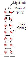
Note that Miranda and Taghavi¡¯s model (2005) is a continuum model. To simulate the nonlinear behavior and damage on different stories of a building, their proposed continuum beams must be discretized. Specifically, each story is discretized into a nonlinear shear spring and a nonlinear flexural spring, which are connected to each other by rigid links, as shown in Figure 1(b). According to the work of Paulay and Priestley (1992), in a RC frame-shear wall structure, the frame primarily exhibits a shear deformation mode which can be represented by shear springs; whereas the shear wall exhibits a flexural deformation mode which can be simulated by flexural springs. Therefore, the elastic and nonlinear properties of the flexural and shear springs are regulated by the properties of the shear wall and frame, respectively.

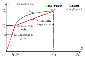
In previous studies, bi-linear and tri-linear curves have been most commonly used to simulate the backbone of inter-story hysteretic behaviors. In this study, such are also employed to model the backbone curves of the flexural and shear springs, as shown in Figure 2(a). The bi-linear backbone curve contains fewer parameters, which is easy to calibrate and has been widely applied (Fajfar and Gaspersic 1996; FEMA 1997). The tri-linear backbone curve, on the other hand, contains more parameters to calibrate but is more capable of representing various nonlinear behaviors. A comparison of the two backbone curves is discussed in Section 4.2 of this work.

The P-D effect normally increases the overturning moment and reduces the lateral resistance of structures. However, the work of Tremblay et al. (2001) indicates that the P-D effect is negligible when the inter-story drift ratio is less than 1/50. According to the Chinese seismic design code (MOHURD 2010b), the inter-story drift ratio should be smaller than 1/100 for RC shear wall or RC frame-shear wall structures subjected to the maximum considered earthquake (MCE) level ground motions. Therefore, the P-D effect is not significant in this work. For stronger earthquakes, where the P-D effect must not be neglected, the method of Gupta and Krawinkler (2000) can be used by incorporating a softening stiffness to the backbone curve.

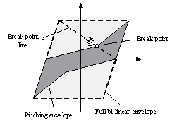
Due to limited amount of detailed building information for urban seismic simulations, a single parameter-pinching model proposed by Steelman and Hajjar (2009) is adopted herein (Figure 2(b)). The pinching parameter can be calibrated based on the structural type, as presented in Section 3.4.

Figure 1. Comparison of the elastic continuum and nonlinear flexural-shear models

(a) The elastic continuum model proposed by Miranda and Taghavi (2005)

(b) NMFS model proposed in this study

Figure 1. Comparison of the elastic continuum and nonlinear flexural-shear models

Figure 2. Inter-story hysteretic model

(a) Bi-linear and tri-linear backbone curves

(b) Single parameter pinching model

Figure 2. Inter-story hysteretic model

3 Parameter calibration based on building attribute data

Given that urban areas cover a large number of tall buildings and that the detailed design information of each building is not easily accessible, the greatest challenges in using the NMFS model for regional seismic simulations are: (a) how to collect the building information in the target area; and (b) how to determine the parameters of the flexural and shear springs. Note that the GIS data of buildings in an urban area are relatively easy to access. Note also that the GIS data contains the building attribute data, such as the structural height, site condition, year of construction and structural type. Therefore, these building attribute data are used in this study to calibrate the parameters of the NMFS model. It should also be mentioned that if the design details of a building (e.g., design drawing) are available, the parameters of the flexural and shear springs can be determined using the method proposed by Kuang and Huang (2011).

Considering limited information in the building attribute data, an accurate determination of the nonlinear parameters of a number of tall buildings is rather challenging. One of the major objectives of this work is to propose a rational parameter determination method for tall buildings. Therefore, this work adopts the fundamentals of the HAZUS method (FEMA 2012a) to determine the inter-story relationships. Specifically, the design strength is determined first, and based on which, other parameters of the backbone curve are also determined. Note that tall buildings are in general thoroughly designed, so that the design strength of a building can be obtained with considerable certainty even if very limited building attribute data are available. The uncertainty of the backbone curve parameters relies mainly on the overstrength factors, displacement parameters and hysteretic parameters. Constrained by the available building attribute data, this work attempts to use as many authoritative literatures as possible to reduce the estimation uncertainty. For example, the HAZUS method (FEMA 2012a) was used to determine the overstrength factors, ductility factor and hysteretic parameters; ACI 318 (ACI Committee 2008) was used to determine the stiffness reduction factor. Note that one of the major contributions of this work is to establish a general framework. Different users from different regions can determine the corresponding parameters based on different local conditions following the proposed framework, should they have more reliable data source.

The model calibration should target RC frame-shear wall dual system structures in this study. Other structural types, such as braced frame structures, can also be calibrated following a similar process.

The entire calibration process displayed in Figure 3 consists of the following four steps: (1) calibration of the elastic parameters, (2) calibration of the yield point, (3) calibration of the peak point, and (4) calibration of the hysteretic parameter.

Figure 3. Illustration of the calibration process

Figure 3. Illustration of the calibration process

3.1 Calibration of the elastic parameters

Miranda and Taghavi¡¯s work (2005) indicates that the influence of the stiffness variation along the building height on its dynamic properties is small and can be neglected. To simplify the calibration process, the stiffness is assumed uniform along the height of the building. Consequently, only two parameters (i.e., the shear and flexural stiffnesses) must be determined for calibration and the first and second modal periods are chosen as inputs for this purpose. Note that the proposed model is suitable for regular buildings. For buildings with highly irregular layout along the height, a more specific modeling method must be proposed.

The first and second periods of a structure can be acquired using the following approaches: (1) modal analyses are always performed for tall buildings during the structural design stage so that the calculated modal periods can be directly adopted; (2) seismic instrumentation is installed in some tall buildings, and monitoring results can be used to obtain the vibration periods; and (3) for other tall buildings in which the former two methods cannot be used, empirical equations can be adopted to determine the first and second periods of a structure. For example, the first period of a RC frame-shear wall structure can be determined using the general form of the empirical period formula recommended by ASCE/SEI 7-10 (ASCE 2010), as shown in Equation 1. The parameters Ct and x can be determined according to the specific condition of the region concerned. In this work, the parameters recommended by Gao and Liu (2012) (Ct = 0.03, x = 0.9) is used to estimate the first period of Chinese buildings. The second period, T2, can be calculated using the empirical relationship given in Equation 2 (Lagomarsino 1993), which is established based on the periods of 52 RC buildings. This empirical equation has also been widely adopted by some other studies to predict the periods of RC dual systems or shear wall buildings (Campbell et al. 2005; Areemit et al. 2012; Williams 2014; Gilles and McClure 2012; Su et al. 2008).

                                                                                                                                              (1)

                                                                                                                                           (2)

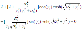
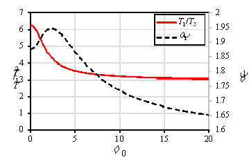
After obtaining T1 and T2, Equations 3 and 4, proposed by Miranda and Taghavi (2005), can be used to calculate a0, which represents the flexural-shear stiffness ratio and is given by Equation 5. gi is the eigenvalue parameter associated with the ith mode of vibration as a function of the nondimensional parameter a0. Hence, once a period ratio is given, the value of alpha can be determined. Note that it is more convenient to determine the periods T1 and T2, the ratio of T1/T2 is thus used to calculate the value of alpha. The relationship between T1/T2, first mode eigenvalue parameter g1 and a0 is shown in Figure 4.

Subsequently, the flexural stiffness EI can be determined using Equation 6, where g1 is calculated from Equation 4 or Figure 4. Finally, Equation 5 is used to calculate the shear stiffness GA.

                                                                                                                                (3)

                                                                                        (4)

                                                                                                                                        (5)

                                                                                                                         (6)

Figure 4. Relationships between T1/T2, g1 and a0

Figure 4. Relationships between T1/T2, g1 and a0

3.2 Calibration of the yield parameters

According to the HAZUS Technical Report (FEMA 2012a), the tri-linear backbone of a capacity curve can be determined using the following three control points: (1) the design strength point, (3) the yield strength point, and (3) the peak strength point. They are presented in Figure 5. The design strength point is the nominal strength determined through the seismic design process (Paulay and Priestley 1992; ASCE 2010; MOHURD 2010b; CEN 2004). The yield strength represents the true lateral strength of the building considering redundancies in design, conservativeness of code requirements and true strength of materials. The peak strength point denotes the maximum lateral strength that accounts for the overstrength effects of the materials. Moreover, the ultimate strength, corresponding to the strength at the collapse-prevention state, equals the peak strength according to the backbone curve proposed by HAZUS. Note that because modern tall buildings are always strictly designed following the seismic design codes, collapse of such buildings is more or less prevented during earthquakes. Therefore, the collapse simulation of tall buildings is not covered in this study, which implies that the determination of the ultimate displacement (i.e., Du in Figure 5) corresponding to the collapse of the building will not be discussed.

The tri-linear backbone curve illustrated in Figure 5 can also be adopted for the flexural and shear springs shown in Figure 1(b). To obtain the yield strength of the tri-linear backbone curve of each spring, the design codes are used first to calculate the nominal seismic forces of each spring. Subsequently, the yield strength is determined by multiplying the nominal seismic forces with the yield overstrength ratio (FEMA 2012a).

Figure 5. Tri-linear backbone curve of HAZUS

Figure 5. Tri-linear backbone curve of HAZUS

The equivalent lateral force analysis (ELFA) and the modal response spectrum analysis (MRSA) are often used to determine the seismic force on each story of a building structure (Paulay and Priestley 1992; ASCE 2010; MOHURD 2010b; CEN 2004). The MRSA is also adopted herein considering the significant contributions of high-order vibrations to the seismic responses of tall buildings. Detailed process is described as follows.

 (1) Perform modal analysis using the elastic parameters obtained in Section 3.1 to calculate the modal shapes fj, n, where j and n are the story and mode number, respectively.

 (2) Perform response spectrum analyses and acquire the spectrum displacement Dn of each mode.

 (3) Calculate the inter-story displacements and rotation based on the mode shape fj, n and spectrum displacement Dn using Equations 7-10.

                                                                                                                                       (7)

                                                                                                                                 (8)

                                                                                                                                      (9)

                                                                                                                              (10)

where uj, n/Duj, n and qj, n/Dqj, n denote the total displacement/inter-story displacement and the total rotation/inter-story rotation, respectively, on the jth story for the nth mode. Note that uj-1,n = 0 and qj-1,n = 0 when j = 1, z is the coordinate along the height of the building.

(4) Calculate the inter-story shear force, Vj, n, in the shear springs and the bending moment, Mj, n, in the flexural springs on each story for each mode using Equations 11 and 12, where hj is the height of the jth story

                                                                                                                                (11)

                                                                                                                              (12)

(5) Combine the modal shear forces in the shear springs and the modal bending moments in the flexural springs on each story for each mode using the square root of the sum of the squares (SRSS) method, as stated in Equations 13 and 14.

                                                                                                                                    (13)

                                                                                                                                 (14)

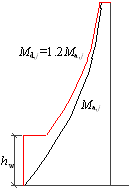
(6) The shear force Va, j and bending moment Ma, j demands of the shear/flexural springs on each story are obtained using MRSA. Such values should be adjusted based on the specifications in the design codes to obtain the actual design capacities. According to the Chinese Technical Specification for Concrete Structures of Tall Buildings (JGJ3-2010) (MOHURD 2010a), the shear force Va, j on each story should be adjusted according to Equation 15 to ensure that the frames (i.e., the shear springs) have sufficient capacities to resist seismic forces after the yield of the shear walls. Similarly, the bending moment Ma, j on each story is also adjusted to Md, j according to the specifications (JGJ3-2010) (MOHURD 2010a) to consider the uncertainties in the analysis and post-elastic dynamic effects, as shown in Figure 6. Specifically, for the stories within the height of the bottom strengthening zone hw, which can be determined according to Equation 16 from Provision 7.1.4 of the Specification (MOHURD 2010a), their bending moments are identical to that at the building base. For the stories located above the bottom strengthening zone, the bending moment obtained through analysis is enlarged by a factor of 1.2 according to Provision 7.2.5 of the Specification (MOHURD 2010a).

                                                                                                                     (15)

                                                                                                                     (16)

where Vbase is the total shear force at the building base, and hstory and hwall are the story height and the total heights of the shear wall, respectively.

Figure 6. Design envelope of bending moment in shear walls

Figure 6. Design envelope of bending moment in shear walls

The above six-step procedure yields the design inter-story shear force Vd, j and the design inter-story bending moment Md, j. The yield overstrength factor Wy is used to estimate the actual yield strength. Specifically, Equations 17 and 18 are adopted to calculate the yield shear strength Vy, j and the yield bending strength My, j. The corresponding yield displacement,  and rotation, can be determined according to Equations 19 and 20, respectively.

                                                                                                                                       (17)

                                                                                                                                   (18)

                                                                                                                                    (19)

                                                                                                                                  (20)

No authoritative discussion is available in the literature on the overstrength factor of Chinese RC frame-shear wall structures. Note that the design philosophy for RC components specified in the Chinese and US codes is very similar (ACI Committee 2008; MOHURD 2010c). Further, Lu et al. (2015) have compared the seismic resistance of two typical RC tall buildings designed following the Chinese and US codes under similar seismic demand. The pushover results indicate that the peak strengths of the two buildings are similar. Therefore, the yield overstrength factor Wy and the peak overstrength factor Wp in Equations 21 and 22 can be determined from Table 5.5 of the HAZUS Technical Report (FEMA 2012a) for the Chinese buildings. Note that this work presents a general framework. The readers can determine the parameters considering their own specific conditions, should they have more reliable data source.

3.3 Calibration of the peak point

The strength and the displacement at the peak point are calibrated during this process. The peak strength can be determined following Equations 21 and 22, where Wp is the overstrength factor given by Table 5.5 of the HAZUS Technical Report (FEMA 2012a) which varies for different types of structures. For example, the value of Wp for RC frame-shear wall structures (i.e., C2H) is 2.5.

                                                                                                                                       (21)

                                                                                                                                    (22)

For the bi-linear backbone curve, in which only the peak point is needed at the turning point of the capacity curve, the peak displacement can be determined using the original stiffness and peak strength as shown in Equations 23 and 24.

                                                                                                                                     (23)

                                                                                                                                  (24)

The peak displacements of tri-linear backbone curve can be calculated using two different methods, viz. (1) the stiffness reduction method, and (2) the ductility factor method. These two methods are discussed as follows.

(1) Stiffness reduction method

The stiffness of a structure is normally reduced due to concrete cracking. The displacement corresponding to the peak strength can be predicted using the reduced bending stiffness ErI and shear stiffness GrA (ACI Committee 2008), using Equations 25 and 26, respectively. The stiffness reduction factor h  can be determined according to Provision 10.10.4.1 of ACI 318-08 (ACI Committee 2008). Subsequently, Equations 27 and 28 can be used to calculate the peak displacements Dup, j and the peak rotation Dqp, j, where Vp, j and Mp, j are respectively the peak strengths of the shear forces in the shear springs and those of the bending moments in the flexural springs on the jth story.

                                                                                                                                           (25)

                                                                                                                                         (26)

                                                                                                                                     (27)

                                                                                                                                   (28)

(2) Ductility factor method

The Hazus Technical Report (FEMA 2012a) also defines the ductility factor m  (see Equation 29), which can be used to calculate the peak displacements, as shown in Equations 30 and 31. The values of m for different structural types can be determined using Table 5.6 of the HAZUS Technical Report (FEMA 2012a).

                                                                                                                                          (29)

                                                                                                                               (30)

                                                                                                                              (31)

The simulation results of the above two peak displacement determination methods are compared in Section 4.2.

3.4 Calibration of the hysteretic parameter

The energy dissipation capacity of a structure is largely influenced by the hysteretic model. For the convenience of the calibration process, the single-parameter hysteretic model proposed by Steelman and Hajjar (2009) is adopted in this study, in which only one parameter t  must be determined. t  is calculated using Equation 32, where Ap and Ab are, respectively, the areas enclosed by the pinching envelope and that under the full bi-linear envelope (see Figure 2(b)). The value of t can be easily calculated using the degradation factor ¦Ê given in Table 5.18 of the HAZUS Technical Report (FEMA 2012a) together with the work of Steelman and Hajjar (2009).

                                                                                                                                                (32)

4 Validation and application of the proposed model to individual building structures

To validate the proposed model and the associated parameter calibration method, the NMFS models of two tall buildings are established and the predicted seismic responses are compared with those of the refined FE models, as presented in Figure 7. Building A is a 15-story RC frame-shear wall structure (see Figure 7(a)), details of which can be found in Ren et al. (2015). Building B is a 42-story RC frame core-tube building (i.e., Building 2N in Lu et al. (2015)), as shown in Figure 7(b). These two buildings are selected because such types of structures are widely used and representative. The RC frame-shear wall structure is commonly used for apartments and hotels, whereas the RC frame core-tube structure is popularly used for offices and commercial centers. The attribute data of the two buildings are listed in Table 1.

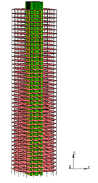
The refined FE models of the two buildings (Figure 7) are established using the general purpose FE software MSC.MARC, in which shear walls and frames are modeled with multi-layer shell elements and fiber beam elements (Lu et al. 2013a). The total numbers of elements are 25,238 and 36,547, respectively, for Buildings A and B. The modeling details and the accuracy of the refined FE model have already been discussed in the work of Ren et al. (2015) and Lu et al. (2015).

Figure 7. Illustration of the refined FE models

(a) Building A (15-story RC frame-shear wall structure)

(b) Building B (42-story RC frame core-tube structure)

Figure 7. Illustration of the refined FE models

Table 1. Building attribute data

Name

Number of stories

Height

Site condition

Year of construction

Structural type

Building A

15

54.9m

Class II

2013

RC frame-shear wall

Building B

42

141.8m

Class II

2013

RC frame core-tube

4.1 Demonstration of the calibration process

The parameters of the NMFS model of Building A in the y-direction (i.e., the direction of the first vibration mode) are used to demonstrate the calibration process. Note that the first and second periods in the y-direction of Building A have already been obtained through modal analysis of the refined FE model during the design stage. The flexural and shear stiffnesses are calculated following the procedures outlined in Section 3.1. Subsequently, modal analysis of the NMFS model is performed, and the resulting vibration periods are compared with those of the refined FE model as shown in Table 2. A good agreement is obtained, as also confirmed by Miranda and Taghavi (2005).

Table 2. Comparison of the vibration periods


T1 (s)

T2 (s)

Refined FE model

1.4422

0.3449

NMFS model

1.4421

0.3473

Error

0.0%

-0.7%

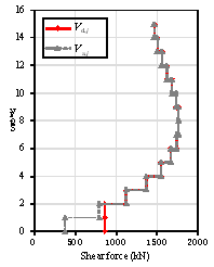
The design response spectrum for MRSA is determined according to the Chinese seismic design code (GB50011-2010) (MOHURD 2010b). Subsequently, the SRSS method is adopted to combine the spectrum responses of different modes. The shear forces in the shear springs and the bending moments in the flexural springs obtained from SRSS are demonstrated as the lines with gray triangles in Figure 8. As discussed in Section 3.2, the shear force and bending moment should be further adjusted according to the design specifications. Additionally, the modified shear forces and bending moments, following the requirements set in Equations 15, 16 and Figure 6, are shown as lines with red diamonds in Figure 8, which represent the design values of Vd, j and Md, j.

The yield strengths Vy, j and My, j and the yield displacements Duy, j and Dqy, j are calculated using Equations 17-20, where Wy = 1.10 for RC frame-shear wall structures (C2H), according to Table 5.5 of the HAZUS Technical Report (FEMA 2012a). The peak strengths Vp, j and Mp, j are calculated according to Equations 21 and 22, with Wu = 2.50 (FEMA 2012a).

As stated in Section 3.3, two methods can be used to determine the peak displacements Duu, j and Dqu, j. If the stiffness reduction method is adopted, the stiffness reduction factor h = 0.7 according to Provision 10.10.4.1 of ACI 318-08 (ACI Committee 2008). If the ductility factor method is adopted, the ductility factor m = 4 according to Table 5.6 of the HAZUS Technical Report (FEMA 2012a). Subsequently, the peak displacements Duu, j and Dqu, j are calculated according to Equations 25-31. The hysteretic parameter t = 0.6 for RC frame-shear wall structures (C2H) according to Table 5.18 of the HAZUS Technical Report (FEMA 2012a).

Figure 8. Design forces on each story

(a) Shear forces in the shear springs

(b) Bending moments in the flexural springs

Figure 8. Design forces on each story

4.2 Comparison of the accuracy of different calculation models

As previously discussed, two backbone curves are available to describe the inter-story hysteretic behavior: (1) bi-linear or (2) tri-linear. In addition, the peak displacements can be determined using either the stiffness reduction method or the ductility factor method. Different combinations of these models/methods are compared to the refined FE model to determine the most accurate prediction method. To demonstrate the advantages of the proposed NMFS model, the elastic continuum model of Miranda and Taghavi (2005) and the NMS model adopted in IES (Hori 2006) are also included in the comparison. A brief summary of different prediction models used for the comparison is provided in Table 3.

Table 3. Comparison of different prediction models

Model name

Model type

Backbone curve

Peak displacement

Parameters

Refined FE model

Multi-layer shell element and fiber beam element

--

--

--

NMFS-Tri-h

Nonlinear MDOF flexural-shear model

Tri-linear backbone

Stiffness reduction method

Wy=1.10 Wp=2.50 h=0.7

NMFS-Tri-m

Nonlinear MDOF flexural-shear model

Tri-linear backbone

Ductility factor method

Wy=1.10 Wp=2.50 m=4

NMFS-Bi

Nonlinear MDOF flexural-shear model

Bi-linear backbone

--

Wy=1.10 Wp=2.50

NMS-Tri-h1

Nonlinear MDOF shear model

Tri-linear backbone

Stiffness reduction method

Wy=1.10 Wp=2.50 h=0.7

Elastic model2

Elastic continuum model

--

--

--

1.   The NMS model is calibrated according to Lu et al.¡¯s work (2014b), where the design inter-story seismic force is identical to that of the NMFS model.

2.   The elastic continuum model of Miranda and Taghavi (2005) is calibrated using the same T1, T2 as the NMFS models.

The widely used ground motion recorded at El-Centro station in the United States in 1940 (PEER 2012) is selected to perform the comparison. To verify the nonlinear capability of the proposed NMFS model, the peak ground acceleration (PGA) is adjusted to 220 gal, which is the intensity of MCE according to the Chinese seismic design code (GB50011-2010) (MOHURD 2010b) for Building A.

4.2.1 Comparison amongst different NMFS models

The base shear-roof displacement curves obtained from the pushover analysis under an inverse triangular load pattern are compared in Figure 9 for Models NMFS-Tri-h, NMFS-Tri-m, NMFS-Bi, and the refined FE model. It is evident that the global base shear-roof displacements of the NMFS models exhibit several turning points, because the shear springs and the flexural springs do not yield simultaneously. Generally, the tri-linear models are in better agreement with the refined FE model than the bi-linear model.
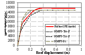
Figure 9. Base shear-roof displacement pushover curves of Models NMFS-Tri-h, NMFS-Tri-m, NMFS-Bi and the refined FE model

Figure 9. Base shear-roof displacement pushover curves of Models NMFS-Tri-h, NMFS-Tri-m, NMFS-Bi and the refined FE model

Subsequently, the nonlinear THA of the four models is performed. Noting that the inter-story drift ratio is one of the most important EDPs for loss estimation, the envelopes of the inter-story drift ratios predicted by the four models are shown in Figure 10. All of the three NMFS models are in good agreement with the refined FE model. This is a most significant outcome because an accurate seismic damage prediction relies heavily on the accuracy of the inter-story drift results. Similar to the finding achieved from Figure 9, the tri-linear models are slightly closer to the refined FE model than the bi-linear model.

Figure 10. Inter-story drift ratios of Models NMFS-Tri-h, NMFS-Tri-m, NMFS-Bi and the refined FE model

Figure 10. Inter-story drift ratios of Models NMFS-Tri-h, NMFS-Tri-m, NMFS-Bi and the refined FE model

4.2.2 Comparison between NMS, Elastic and NMFS models

Although the NMS model can accurately represent the inter-story shear deformation mode of frame structures, it cannot characterize the lateral deformation mode of tall buildings with shear walls. The inter-story drift ratio envelopes of Model NMS-Tri-h, Model NMFS-Tri-h and the refined FE model are compared in Figure 11, which clearly indicates that Model NMS-Tri-h significantly overestimates the inter-story drift ratio of the lower stories and underestimates the inter-story drift ratio of the higher stories. As a result, the NMS model cannot be used for seismic loss estimation of tall buildings because the inter-story drift ratio is a highly important EDP for such an estimation.

The inter-story drift ratio envelopes of Model NMFS-Tri-h, Elastic model and the refined FE model are also compared in Figure 11. As evident in the figure, the result of Elastic model is much smaller than those of the refined FE model and the NMFS models. The two comparisons above show that the prediction of Model NMFS-Tri-h is significantly better.

Figure 11. Inter-story drift ratios of Model NMFS-Tri-h, Model NMS-Tri-h, Elastic model and the refined FE model

Figure 11. Inter-story drift ratios of Model NMFS-Tri-h, Model NMS-Tri-h, Elastic model and the refined FE model

4.2.3 Comparative studies with multiple ground motions

Considering the random nature of earthquakes, multiple ground motions are adopted in this section to further demonstrate the accuracy of the proposed NMFS model. A total of 22 far field ground motions recommended by FEMA-P695 (FEMA 2009), which are widely used in many related studies, are input into the refined FE models and the NMFS models of the two tall buildings. The PGAs are set to 220 gal and 510 gal for Buildings A and B, respectively, corresponding to their MCE levels specified in the Chinese seismic design code (GB50011-2010) (MOHURD 2010b).

The predicted maximum inter-story drift ratios of Building A subjected to different ground motions are compared in Figure 12 using the three NMFS models (i.e., Model NMFS-Tri-h, Model NMFS-Tri-m and Model NMFS-Bi) and the refined FE model. As evident in Figure 12, though the maximum inter-story drift ratios vary significantly under different ground motions due to their randomness (Lu et al. 2013c; Lu et al. 2013d), the predicted maximum inter-story drift ratios of all three NMFS models generally agree well with those of the refined FE model, which confirms the robustness of the proposed model. In addition, the seismic responses show significant nonlinearity. The average ratio of the maximum inter-story displacement to the yield inter-story displacement under the 22 ground motions is 5.9. Results also indicate that Model NMFS-Tri-h has the smallest average error, which is followed by Model NMFS-Tri-m. The average error of Model NMFS-Bi is the largest. Such conclusion is similar to the findings obtained from Figures 9 and 10. In view of this, Model NMFS-Tri-h and Model NMFS-Tri-m are recommended for the regional seismic simulation.
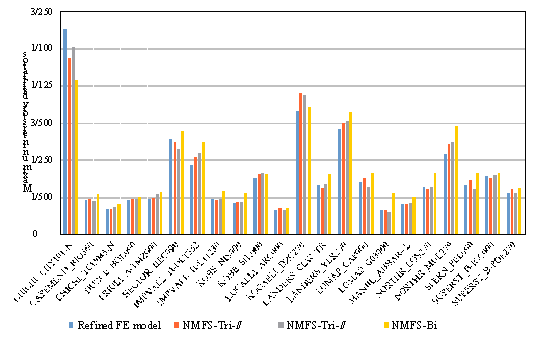
Figure 12. Predicted maximum inter-story drift ratios of Building A subject to the 22 ground motions

Figure 12. Predicted maximum inter-story drift ratios of Building A subject to the 22 ground motions

The average inter-story drift ratios along the height of the two buildings subject to the 22 ground motions are presented in Figure 13. The results of both Model NMFS-Tri-m and Model NMFS-Tri-h are in good agreement with those of the refined FE model. Given that rather limited information is required to calibrate the parameters in the proposed NMFS model, the accuracies of the NMFS model and the associated parameter calibration method are considered acceptable. Note, for Building A, that the computational time using the NMFS model subjected to the 22 ground motions is only 135 CPU seconds on a desktop computer (CPU: 2.67-GHz Intel Xeon X5650, RAM: 48GB of 1333-MHz DDR3), whilst the refined FE model takes 1137 CPU hours. The speedup ratio of 30,320 (= 1137 ¡Á 3600 ¡Â 135) confirms a remarkable efficiency of the proposed NMFS model.

Figure 13. Average inter-story drift ratios for Buildings A and B subject to the 22 ground motions

(a) Building A

(b) Building B

Figure 13. Average inter-story drift ratios for Buildings A and B subject to the 22 ground motions

5 Application of the proposed method to regional buildings

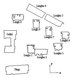
A residential area in China covering nine tall RC frame-shear wall buildings and two medium-rise RC frame buildings is investigated to demonstrate the applicability of the proposed model for regional areas. The GIS data are presented in Table 4 and Figure 14. The nine tall buildings are analyzed using the NMFS model proposed in this work, and the two medium-rise buildings are simulated with the NMS model according to the work of Lu et al. (2014b).

A nonlinear time-history analysis of this region is implemented subject to El-Centro EW ground motion in the x-direction with PGA = 400 gal (i.e., the MCE level ground motion of this region). The seismic displacement responses at the time step t = 10 s are shown in Figure 15(a). The entire time-history analysis consumes 261 CPU seconds on a desktop computer (CPU: 2.67-GHz Intel Xeon X5650, RAM: 48GB of 1333-MHz DDR3) which demonstrates a high computational efficiency. As demonstrated in Figure 15(b), the envelope of inter-story drift ratios of each building can be calculated and displayed, which is critical for seismic loss estimations.

Table 4. Building inventory

Label

Name of building

Number of stories

Height

(m)

Site condition

Year of construction

Structural type

1

Yingu

23

92

Class II

2000

RC frame-shear wall

2

Caizhi

28

112

Class II

1998

RC frame-shear wall

3

Longhu-1

27

108

Class II

2010

RC frame-shear wall

4

Longhu-2

9

36

Class II

2010

RC frame-shear wall

5

Longhu-3

25

100

Class II

2010

RC frame-shear wall

6

Longhu-4

19

76

Class II

2010

RC frame-shear wall

7

Longhu-5

7

28

Class II

2010

RC frame

8

Longhu-6

7

28

Class II

2010

RC frame

9

Longhu-7

18

72

Class II

2010

RC frame-shear wall

10

Longhu-8

19

76

Class II

2010

RC frame-shear wall

11

Longhu-9

15

60

Class II

2010

RC frame-shear wall


Figure 14. 2D-GIS plan of buildings in a regional area

Figure 14. 2D-GIS plan of buildings in a regional area

Figure 15. Seismic response results of buildings in a regional area

(a) Displacements
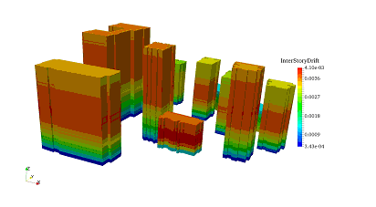
Figure 15. Seismic response results of buildings in a regional area

(b) Envelopes of inter-story drift ratios

Figure 15. Seismic response results of buildings in a regional area

6 Conclusions

A nonlinear MDOF flexural-shear (NMFS) model and the associated parameter calibration method are proposed for the regional seismic damage analyses of tall buildings. The NMFS model has several advantages, including (1) the representation of the flexural-shear deformation mode of tall buildings, (2) a high computational efficiency, (3) convenient and efficient parameter calibration and (4) the ability to output the inter-story drift on each story. By comparing with the widely used NMS model, the proposed NMFS model is capable of simulating the flexural-shear deformation characteristics of tall buildings more realistically, and the accuracy of the predicted inter-story drift is significantly improved. Meanwhile the computational efficiency is also remarkably enhanced compared with that of the corresponding refined FE model. In addition, the parameter calibration method is easy to implement, which only requires widely accessible building attribute data.

Different calibration approaches are compared, indicating that the tri-linear backbone curve performs better than the bi-linear backbone curve. Both the stiffness reduction method and the ductility factor method demonstrate acceptable accuracies. Finally, the seismic damage to an urban area of tall buildings is simulated using the proposed model. The computational efficiency is reasonably high for a large-scale regional seismic analysis. Overall, this study may facilitate future high-fidelity regional seismic loss estimations of tall buildings.

Acknowledgements The authors are grateful for the financial support received from the National Key Technology R&D Program (Nos. 2015BAK17B03), the National Natural Science Foundation of China (No. 51578320), the National Non-profit Institute Research Grant of IGP-CEA (Grant No: DQJB14C01) and the European Community's Seventh Framework Programme, Marie Curie International Research Staff Exchange Scheme (IRSES) under grant agreement n¡ã 612607.

References

ACI Committee (2008) Building code requirements for structural concrete (ACI 318-08) and Commentary (318R-08). American Concrete Institute, Farmington Hills, Michigan

Areemit N, Montgomery M, Christopoulos C, Hasan A (2012) Identification of the dynamic properties of a reinforced concrete coupled shear wall residential high-rise building. Can J Civ Eng 39(6):631-642

ASCE (2010) Minimum design loads for buildings and other structures (ASCE/SEI 7-10). American Society of Civil Engineers, Reston, Virginia

Campbell S, Kwok KCS, Hitchcock PA (2005) Dynamic characteristics and wind-induced response of two high-rise residential buildings during typhoons. J Wind Eng Ind Aerodyn 93(6):461-482

CEN (2004) Eurocode 8: Design of structures for earthquake resistance. Part 1: General rules, seismic action and rules for buildings. Comite Europeen de Normalisation, Brussels

Fajfar P, Gaspersic P (1996) The N2 method for the seismic damage analysis for RC buildings. Earthq Eng Struct Dyn 25(1):23-67

FEMA (1997) NEHRP guidelines for the seismic rehabilitation of buildings (FEMA-273). Federal Emergency Management Agency, Washington, DC

FEMA (2009) Quantification of building seismic performance factors (FEMA P695). Federal Emergency Management Agency, Washington, DC

FEMA (2012a) Multi-Hazard loss estimation methodology-earthquake model technical manual (HAZUS-MH 2.1). Federal Emergency Management Agency, Washington, DC

FEMA (2012b) The seismic performance assessment of buildings, volume 1 methodology (FEMA P-58-1). Prepared by the Applied Technology Council for the Federal Emergency Management Agency, Washington, DC

Gao YQ, Liu WF (2012) Statistical analysis of fundamental periods of frame-shear wall structures. Appl Mech Mater 174-177:2071-2078

Gilles D, McClure G (2012) Measured natural periods of concrete shear wall buildings: insights for the design of Canadian buildings. Can J Civ Eng 39(8):867-877

Gu¨¦guen P, Michel C, LeCorre L (2007) A simplified approach for vulnerability assessment in moderate-to-low seismic hazard regions: application to Grenoble (France). Bull Earthquake Eng 5(3):467-490

Gupta A, Krawinkler H (2000) Dynamic P-delta effects for flexible inelastic steel structures. J Struct Eng 126(1):145-154

Hori M (2006) Introduction to computational earthquake engineering. Imperial College Press, London

Ibarra LF, Krawinkler H (2005). Global collapse of frame structures under seismic excitations. Pacific Earthquake Engineering Research Center, California

Krawinkler H, Medina R, Alavi B (2003) Seismic drift and ductility demands and their dependence on ground motions. Eng Struct 25(5):637-653

Kuang JS, Huang K (2011) Simplified multi-degree-of-freedom model for estimation of seismic response of regular wall-frame structures. Struct Des Tall Spec Build 20(3):418-432

Lagomarsino S (1993) Forecast models for damping and vibration periods of buildings. J Wind Eng Ind Aerod 48(2-3):221-239. doi:10.1016/0167-6105(93)90138-E

Lu X, Lu XZ, Guan H, Ye LP (2013a) Collapse simulation of reinforced concrete high-rise building induced by extreme earthquakes. Earthq Eng Struct Dyn 42(5):705-723

Lu XZ, Lu X, Guan H, Zhang WK, Ye LP (2013b) Earthquake-induced collapse simulation of a super-tall mega-braced frame-core tube building. J Constr Steel Res 82:59-71

Lu X, Lu XZ, Guan H, Ye LP (2013c) Comparison and selection of ground motion intensity measures for seismic design of super high-rise buildings. Adv Struct Eng 16(7):1249¨C1262

Lu X, Ye LP, Lu XZ, Li MK, Ma XW (2013d) An improved ground motion intensity measure for super high-rise buildings. Sci China Technol Sc 56(6):1525¨C1533

Lu X, Lu XZ, Sezen H, Ye LP (2014a) Development of a simplified model and seismic energy dissipation in a super-tall building. Eng Struct 67:109-122

Lu XZ, Han B, Hori M, Xiong C, Xu Z (2014b) A coarse-grained parallel approach for seismic damage simulations of urban areas based on refined models and GPU/CPU cooperative computing. Adv Eng Softw 70:90-103

Lu XZ, Li MK, Guan H, Lu X, Ye LP (2015) A comparative case study on seismic design of tall RC frame©\core©\tube structures in China and USA. Struct Des Tall Spec Build 24(9):687-702

MAE Center (2006) Earthquake risk assessment using MAEviz 2.0: a tutorial. Mid-America Earthquake Center, University of Illinois at Urbana-Champaign, Urbana-Champaign, Illinois

Miranda E, Taghavi S (2005) Approximate floor acceleration demands in multistory buildings. I: Formulation. J Struct Eng 131(2):203-211

MOHURD (2010a) Technical specification for concrete structures of tall building (JGJ3-2010). Ministry of Housing and Urban-Rural Development of the People¡¯s Republic of China, Beijing

MOHURD (2010b) Code for seismic design of buildings (GB50011-2010). Ministry of Housing and Urban-Rural Development of the People¡¯s Republic of China, Beijing

MOHURD (2010c) Code for design of concrete structures (GB50010-2010). Ministry of Housing and Urban-Rural Development of the People¡¯s Republic of China, Beijing

Nakashima M, Ogawa K, Inoue K (2002) Generic frame model for simulation of earthquake responses of steel moment frames. Earthq Eng Struct Dyn 31(3):671-692

Paulay T, Priestley MJN (1992) Seismic design of reinforced concrete and masonry buildings. John Wiley, New York

PEER (2012) PEER NGA Database. Pacific Earthquake Engineering Research Center. http://peer.berkeley.edu/nga/. Accessed on 2 October 2015

Reinoso E, Miranda E (2005) Estimation of floor acceleration demands in high-rise buildings during earthquakes. Struct Des Tall Spec Build 14(2):107-130

Ren PQ, Li Y, Guan H, Lu XZ (2015) Progressive collapse resistance of two typical high-rise RC frame shear wall structures. ASCE J Perform Constr Facil 29(3): 04014087. doi: 10.1061/(ASCE)CF.1943-5509.0000593

Reyners M (2011) Lessons from the destructive Mw 6.3 Christchurch, New Zealand, earthquake. Seismol Res Lett 82(3):371-372

Steelman JS, Hajjar JF (2009) Influence of inelastic seismic response modeling on regional loss estimation, Eng Struct 31(12):2976-2987

Su RKL, Lam NTK, Tsang HH (2008) Seismic drift demand and capacity of non-seismically designed concrete buildings in Hong Kong. Electron J Struct Eng 8:110-121

Tremblay R, L¨¦ger P, Tu J (2001) Inelastic seismic response of concrete shear walls considering P-delta effects. Can J Civ Eng 28(4):640-655

Wang MF, Zhou XY (2002) A practical method for nonlinear seismic responses of RC frame wall structure. China Civil Engineering Journal 35(6):32-38 (in Chinese)

Wikipedia (2012) List of tallest buildings in Christchurch. http://en.wikipedia.org/wiki/List_of_tallest_buildings_in_Christchurch. Accessed on 2 October 2015

Wilkinson S, Grant D, Williams E, Paganoni S, Fraser S, Boon D, Mason A, Free M (2013) Observations and implications of damage from the magnitude Mw 6.3 Christchurch, New Zealand earthquake of 22 February 2011. Bull Earthquake Eng 11(1):107-140

Williams SS (2014) Modernizing the system hierarchy for tall buildings: a data-driven approach to system characterization. Master dissertation, University of Notre Dame, Notre Dame, Indiana


C. Xiong

Key Laboratory of Civil Engineering Safety and Durability of China Education Ministry, Department of Civil Engineering, Tsinghua University, Beijing 100084, China

X.Z. Lu (Corresponding author)

Key Laboratory of Civil Engineering Safety and Durability of China Education Ministry, Department of Civil Engineering, Tsinghua University, Beijing 100084, China

E-mail: luxz@tsinghua.edu.cn

H. Guan

Griffith School of Engineering, Griffith University, Gold Coast Campus, Queensland 4222, Australia

Z. Xu

School of Civil and Environmental Engineering, University of Science and Technology Beijing, Beijing 100083, China.

Introduction
Research
Application
Teaching
Publications
Download
Issues
Others


Our Lab

Collapse Prevention Committee